14.7 - Ward’s Method
14.7 - Ward’s MethodThis is an alternative approach for performing cluster analysis. Basically, it looks at cluster analysis as an analysis of variance problem instead of using distance metrics or measures of association.
This method involves an agglomerative clustering algorithm. It will start out at the leaves and work its way to the trunk, so to speak. It looks for groups of leaves that form into branches, the branches into limbs, and eventually into the trunk. Ward's method starts out with n clusters of size 1 and continues until all the observations are included in one cluster.
This method is most appropriate for quantitative variables and not binary variables.
Based on the notion that clusters of multivariate observations should be approximately elliptical in shape, we assume that the data from each of the clusters have been realized in a multivariate distribution. Therefore, it would follow that they would fall into an elliptical shape when plotted in a p-dimensional scatter plot.
Let \(X _ { i j k }\) denote the value for variable k in observation j belonging to cluster i.
Furthermore, we define:
We sum over all variables and all of the units within each cluster. We compare individual observations for each variable against the cluster means for that variable.
The total sums of squares are defined the same as always. Here we compare the individual observations for each variable against the grand mean for that variable.
This \(r^{2}\) value is interpreted as the proportion of variation explained by a particular clustering of the observations.
- Error Sum of Squares: \(ESS = \sum_{i}\sum_{j}\sum_{k}|X_{ijk} - \bar{x}_{i\cdot k}|^2\)
- Total Sum of Squares: \(TSS = \sum_{i}\sum_{j}\sum_{k}|X_{ijk} - \bar{x}_{\cdot \cdot k}|^2\)
- R-Square: \(r^2 = \frac{\text{TSS-ESS}}{\text{TSS}}\)
Using Ward's Method we start out with all sample units in n clusters of size 1 each. In the first step of the algorithm, n - 1 clusters are formed, one of size two and the remaining of size 1. The error sum of squares and \(r^{2}\) values are then computed. The pair of sample units that yield the smallest error sum of squares, or equivalently, the largest \(r^{2}\) value will form the first cluster. Then, in the second step of the algorithm, n - 2 clusters are formed from that n - 1 clusters defined in step 2. These may include two clusters of size 2 or a single cluster of size 3 including the two items clustered in step 1. Again, the value of \(r^{2}\) is maximized. Thus, at each step of the algorithm, clusters or observations are combined in such a way as to minimize the results of error from the squares or alternatively maximize the \(r^{2}\) value. The algorithm stops when all sample units are combined into a single large cluster of size n.
Example 14-3: Woodyard Hammock Data (Ward's Method)
We will take a look at the implementation of Ward's Method using the SAS program below. Minitab implementation is also similar. Minitab is not shown separately.
Download the SAS Program here: wood5.sas
Note: In the upper right-hand corner of the code block you will have the option of copying ( ) the code to your clipboard or downloading ( ) the file to your computer.
options ls=78;
title "Cluster Analysis - Woodyard Hammock - Ward's Method";

 /* After reading in the data, an ident variable is created as the
  * row number for each observation. This is neeed for the clustering algorithm.
  * The drop statement removes several variables not used for this analysis.
  */

data wood;
  infile 'D:\Statistics\STAT 505\data\wood.csv' firstobs=2 delimiter=',';
  input x y acerub carcar carcor cargla cercan corflo faggra frapen
        ileopa liqsty lirtul maggra magvir morrub nyssyl osmame ostvir
        oxyarb pingla pintae pruser quealb quehem quenig quemic queshu quevir
        symtin ulmala araspi cyrrac;
  ident=_n_;
  drop acerub carcor cargla cercan frapen lirtul magvir morrub osmame pintae
       pruser quealb quehem queshu quevir ulmala araspi cyrrac;
  run;

 /* The observations are sorted by their ident value.
  */

proc sort data=wood;
  by ident;
  run;

 /* The cluster procedure is for hierarchical clustering.
  * The method option specifies the cluster distance formula to use.
  * The outtree option saves the results.
  */

proc cluster data=wood method=ward outtree=clust1;
  var carcar corflo faggra ileopa liqsty maggra nyssyl ostvir oxyarb
      pingla quenig quemic symtin;
  id ident;
  run;

 /* The tree procedure generates a dendrogram of the heirarchical
  * clustering results and saves cluster label assignments if the
  * nclusters option is also specified.
  */

proc tree data=clust1 horizontal nclusters=6 out=clust2;
  id ident;
  run;

 /* The data are sorted by their ident value.
  */

proc sort data=clust2;
  by ident;
  run;

 /* This step combines the original wood data set with
  * the results of clust2, which allows the ANOVA statistics
  * to be calculated in the following glm procedure.
  */

data combine;
  merge wood clust2;
  by ident;
  run;

 /* The glm procedure views the cluster labels as ANOVA groups and
  * reports several statistics to assess variation between clusters
  * relative to variation within clusters.
  * The mean for each cluster is also reported.
  */

proc glm data=combine;
  class cluster;
  model carcar corflo faggra ileopa liqsty maggra nyssyl ostvir oxyarb
        pingla quenig quemic symtin = cluster;
  means cluster;
  run;
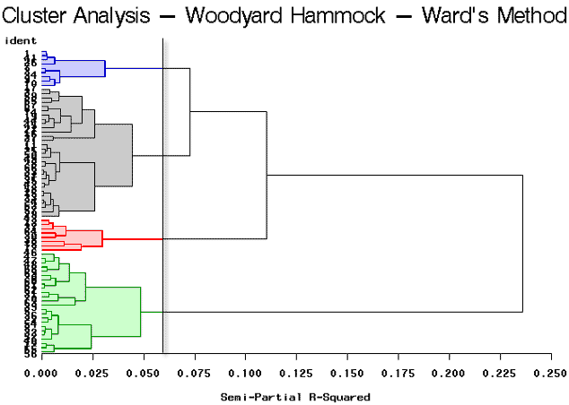
As you can see, this program is very similar to the previous program, (wood1.sas), that was discussed earlier in this lesson. The only difference is that we have specified that method=ward in the cluster procedure as highlighted above. The tree procedure is used to draw the tree diagram shown below, as well as to assign cluster identifications. Here we will look at four clusters.

The break in the plot shows four highlighted clusters. It looks as though there are two very well-defined clusters because it shows a large break between the first and second branches of the tree. The partitioning results in 4 clusters yielding clusters of sizes 31, 24, 9, and 8.
Referring back to the SAS output, the results of the ANOVAs are copied here for discussion.
| Code | Species | F | p-value |
|---|---|---|---|
| carcar | Ironwood | 67.42 | < 0.0001 |
| corflo | Dogwood | 2.31 | 0.0837 |
| faggra | Beech | 7.13 | 0.0003 |
| ileopa | Holly | 5.38 | 0.0022 |
| liqsty | Sweetgum | 0.76 | 0.5188 |
| maggra | Magnolia | 2.75 | 0.0494 |
| nyssyl | Blackgum | 1.36 | 0.2627 |
| ostvir | Blue Beech | 32.91 | < 0.0001 |
| oxyarb | Sourwood | 3.15 | 0.0304 |
| pingla | Spruce Pine | 1.03 | 0.3839 |
| quenig | Water Oak | 2.39 | 0.0759 |
| quemic | Swamp Chestnut Oak | 3.44 | 0.0216 |
| symtin | Horse Sugar | 120.95 | < 0.0001 |
d.f. = 3, 68
We boldfaced the species whose F-values, using a Bonferroni correction, show significance. These include Ironwood, Beech, Holly, Blue Beech, and Horse Sugar.
Next, we look at the cluster Means for these significant species:
| Code | Cluster | |||
|---|---|---|---|---|
| 1 | 2 | 3 | 4 | |
| carcar | 2.8 | 18.5 | 1.0 | 7.4 |
| faggra | 10.6 | 6.0 | 5.9 | 6.4 |
| ileopa | 7.5 | 4.3 | 12.3 | 7.9 |
| ostvir | 5.4 | 3.1 | 18.3 | 7.5 |
| symtin | 1.3 | 0.7 | 1.4 | 18.8 |
Again, we boldfaced the values that show an abundance of that species within the different clusters.
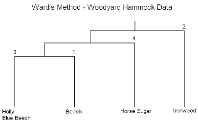
- Cluster 1: Beech (faggra): Canopy species typical of old-growth forests.
- Cluster 2: Ironwood (carcar): Understory species that favors wet habitats.
- Cluster 3: Holly (ileopa) and Blue Beech (ostvir): Understory species that favor dry habitats.
- Cluster 4: Horse Sugar(symtin): Understory species typically found in disturbed habitats.
Note! This interpretation is cleaner than the interpretation obtained earlier from the complete linkage method. This suggests that Ward's method may be preferred for the current data.
The results are summarized in the following dendrogram:

In summary, this method is performed in essentially the same manner as the previous method the only difference is that the cluster analysis is based on the Analysis of Variance instead of distances.