3 Measurements of Disease Occurrence and Frequency
Objectives
Upon completion of this lesson, you should be able to:
- Select and use measures of disease frequency
- Define and calculate point prevalence, period prevalence, cumulative incidence, and incidence density rate
- Describe a potential outbreak with regard to person, place, and time.
- Construct and interpret an epi-curve to describe the course of an outbreak
3.1 Disease Occurrence
Outcomes
Typical outcomes for an epidemiologic study, (sometimes referred to as the ’D’s of Epidemiology) are as follows:
Outcomes of Epidemiology:
- Death Disease/Illness: Physical signs, laboratory abnormalities
- Discomfort: Symptoms (e.g., pain, nausea, dyspnea, itching, tinnitus)
- Disability: Impaired ability to do usual activities
- Dissatisfaction: Emotional reaction (e.g., sadness, anger)
- Destitution Poverty, unemployment
Calculations
In order to describe and compare measures of disease occurrence, these are the types of calculations most often used:
Definition 3.1 (Count) the number of individuals who meet the case definition
Example: 9188 cases of invasive colorectal cancer in Pennsylvania in 2005 (PA Cancer Registry data)
Definition 3.2 (Proportion) \(A/(A+B)\); a fraction in which the numerator \((A)\) includes only individuals who meet the case definition and the denominator, and \((A+B)\) totals the numbers of individuals who meet the case definition \((A)\) plus those in the study population who do not meet the case definition and are at risk \((B)\).
Example: 30% of persons over 50 years of age have been screened for colon cancer
Definition 3.3 (Ratio) \(A/B\); a special fraction in which the numerator includes only individuals who meet one criterion (e.g. the case definition, \(A\)) and the denominator includes only individuals in the study population who meet another criterion (e.g. do not meet the case definition but are at risk, \(B\)).
A ratio is not dependent upon time. If the ratio is a ratio of the number of individuals with the outcome to those without the outcome, the ratio is the odds. A ratio as a measure of disease frequency is used infrequently, in special situations. (not to be confused with an odds-ratio or risk-ratio)
Examples:
- 1 case of colon cancer for every 1 case of breast cancer.
- 2 female cases of major depression to 1 male case of major depression.
Definition 3.4 (Rate) a fraction in which the numerator includes only individuals who meet the case definition and the denominator includes individuals in the study population who do or do not meet the case definition but could meet the case definition (at-risk) and the total time at risk they contribute (person-time). Person-time is defined as the sum of time that each at-risk individual contributes to the study. If the study period is 2 years, person-time is as follows for certain groups:
- For participants who develop the disease
- time they spend on study before they developed the disease (< 2 years)
- These participants count in the numerator, and denominator
- For participants who drop out before 2 year period is over
- time they spend on study before they developed the disease (< 2 years
- These participants count only in the denominator
- For participants who do not develop the disease (in the 2 year window)
- 2 years
- These participants count only in the denominator
The sum of all these times would be the denominator.
Example: 0.1 case/person-years indicates that, on average, for every 10 person-years (i.e.: 10 people each followed 1 year or 2 people followed for 5 years, etc.) contributed, 1 new case of the health outcome will develop
Definition 3.5 (Risk) A measure of the probability of an unaffected individual developing a specified health outcome over a given period of time. Risk is calculated by dividing the number of new cases by the total number of individuals at risk during the specified time period.
Example: A 5-year risk of 0.10 indicates that an individual at risk has a 10% chance of developing the given health outcome in a 5-year period
3.2 Disease Frequency: Incidence vs. Prevalence
The two main ways by which the frequency of disease is measured are incidence and prevalence. These can be distinguished by differences in the time of disease onset.
Definition 3.6 (Incidence) counts new cases of the disease (or outcome)
Definition 3.7 (Prevalence) counts new and existing cases of the disease (or outcome)
Incidence
Incidence quantifies the development of disease. Incidence can be estimated using data from a disease registry data or a cohort trial. There is an implicit assumption of a period of time, such as new cases within a month (or a year).
A summary incidence rate can estimate the risk (e.g., probability of disease in an individual) if the risk is constant across the summarized groups.
As defined, incidence is a count of new cases. However, it is often expressed as a proportion of those at risk. The denominator includes all persons at risk for the disease or condition, i.e. disease-free or condition-free individuals in the population at the start of the time period. Persons in the denominator, those at-risk, should be able to appear in the numerator. Obviously, the denominator would not include persons who already have the disease or condition. Incidence can also be expressed in terms of person-time at risk.
Rates are usually expressed per 100, 1,000, or 100,000 persons. In a strict application, “rate” should only be used when the denominator is an estimate of the total person-time at risk. (You will find the term “rate” used inconsistently in epidemiologic reports. It is better to seek the source of the numbers than to rely on the nomenclature.)
Two Common Measures of Incidence
Definition 3.8 (Cumulative Incidence) The cumulative incidence consists of the number of persons who newly experience the disease or studied outcome during a specified period of time divided by the total population at risk. This calculation assumes all persons in the denominator contribute an equal amount of time to the measure.
Definition 3.9 (Incidence Density Rate) Incidence density rate (also known as incidence rate; person-time rate) is the number of persons who newly experience the outcome during a specified period of time divided by the sum of the time that each member of the population is at-risk.
Prevalence
Since prevalence counts both new and existing cases, the duration of the disease affects the prevalence. Diseases with a long duration will be more prevalent than those with a shorter duration. Chronic, non-fatal conditions are more prevalent than conditions with high mortality. The prevalence of disease is directly related to the duration of the disease. Prevalence is not an apt descriptor of an acute condition.
Similar to incidence, persons included in the denominator must have the potential for being in the numerator, i.e. at-risk for the disease or condition. Prevalence is often expressed after multiplication by 100 (%), 1000, or 100,000.
The prevalence pool is the subset of the population with the condition of interest. The prevalence pool is not generally useful for hypothesis-driven epidemiologic research because these are not new cases, but can be useful in tracking the natural history of the disease, evaluating effects of treatments, or disease burden.
For most etiologic research, incidence is the more appropriate measure. Studying the incidence of a rare condition, however, poses a challenge. Given a small number of new cases, it can be preferable to estimate prevalence instead of incidence in these situations. For example, birth defect rates reported as the number of cases/live births is a prevalent measure. Similarly, an autopsy rate is a prevalent measure.
Two Common Measures of Prevalence
The difference is whether the estimate is made over a period of time or at one specific time as illustrated below:
Definition 3.10 (Point Prevalence) Prevalence of condition of interest at a specific time.
Number of existing cases on a specific date/ Number in the defined population on this date
Point prevalence ranges from 0 to 100. (%)
Point prevalence can be estimated from a cross-sectional survey or disease registry data by calculating the percentage with a particular disease or condition on a particular date.
E.g. what percentage had a particular type of flu on 1/17/2009?
Definition 3.11 (Period Prevalence) Prevalence of outcome of interest during a specified period of time.
Less frequently used.
Number of cases that occurred in a specified period of time/ Number in the defined population during this period
Period prevalence generally ranges from 0 to 100 %. (Theoretically, period prevalence can exceed 100% if you allow individuals who had the disease more than once to be counted for each case of the disease within the reporting period.)
E.g. What percentage of the population had an episode of flu between October and May within the most recent flu season?
3.3 Outbreak Investigation
Investigating a Potential Outbreak
In this course, we have often assumed that investigators have knowledge of a potentially harmful exposure coincidentally with or prior to observing the disease or illness. In other situations, the first indication of harmful exposure is a report of a potential outbreak of disease or illness. Increased numbers of cases of disease or illness may necessitate an outbreak investigation. Questions to be answered in an outbreak investigation include the following:
Are there an unusual number of adverse health outcomes in this community?
If so, how many? Is the number increasing, decreasing, or stable?
What type of exposure may have caused the increase?
What is the anticipated future course and spread of this outbreak?
When an increase in the number of cases of a disease is reported, a speedy response is critical. At the same time, it is also of utmost importance to end up with an answer that will appropriately protect public health and safety. A systematic approach to outbreak investigation helps assure timely and accurate answers:
- Prepare for fieldwork
- Establish the existence of an outbreak
- Verify the diagnosis
- Define and identify cases
- Measure the frequency of adverse outcomes and describe the data in terms of time, place, and person
- Develop hypotheses
- Evaluate hypotheses
- Refine hypotheses and carry out additional studies
- Implement control and prevention measures
- Communicate findings
Orient in Terms of Time, Place, and Person
Characterizing by time: Constructing an Epi-Curve
An epidemic curve, frequently referred to as an ‘epi-curve’, is used to examine and characterize the occurrence of a possible outbreak. By constructing and examining an accurate epi-curve, an investigator can consider questions such as:
Is there an outbreak? If so, when did the outbreak begin?
Has the outbreak peaked? If so, when was the peak?
What might be the source of the exposure? Is there one source or multiple sources for exposure of cases? Is person-to-person transmission occurring?
Have the attempts to control the outbreak coincided with a decrease in the occurrence of the disease?
An epi-curve is a histogram with the number of cases of the adverse health outcome on the y-axis (ordinate) and dates of onset of the outcome on the x-axis (abscissa). Dates of onset may be grouped by days, weeks, or months, depending on the nature of the potential outbreak. A typical time period used is 1/4 to 1/3 the incubation period for the disease. If the incubation or lag time from exposure to outcome is unknown, it is valuable to experiment with different lengths of time.
A typical epi-curve is a simple chart with one series of data, the onset of cases. In other situations, several layers of data are displayed on the curve. For example, the investigator may want to examine the date of onset in more than one location (e.g. 2 or more cities, states, or countries) or in different groups of people (e.g. stratified by age or race).
Another variation of the epi-curve is stacking the bars in order to show different characteristics of the cases. For example, you may decide to separate confirmed cases from suspect cases, using stacked bars to assess whether an outbreak is truly occurring.
Interpreting an Epi-Curve
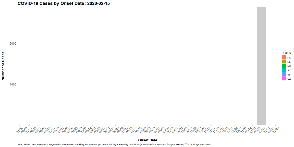
The following shows the outbreak of COVID-19 cases in Pennsylvania:
The first consideration is the overall shape of the curve which is determined by the pattern of the outbreak (common source or person-to-person transmission). The shape also indicates the period of time over which susceptible people are exposed and the minimum, average, and maximum incubation periods for the disease.
If the duration of exposure is prolonged, the epidemic is called a “continuous common source epidemic,” and the epidemic curve will have a plateau instead of a peak. Person-to-person spread (a “propagated” epidemic) should have a series of progressively taller peaks one incubation period apart.
Cases that stand apart (“outliers”) provide valuable information. An early case can represent a background (unrelated) case, a source of the epidemic, or a person who was exposed earlier than others. Similarly, late cases may be unrelated to the outbreak, may have especially long incubation periods, may indicate exposure later than most of the people affected, or may be secondary cases (the person who becomes ill after being exposed to someone who was part of the initial outbreak). Examine any outliers that are part of the outbreak carefully because they may point directly to the source. For example, a prep chef could be the first case of strep in an epidemic among party-goers eating food prepared by this person.
In a point-source epidemic of a disease with a known incubation period, the epidemic curve can also identify the likely period of exposure.
Characterizing by Place
A simple technique for looking at geographic patterns is to plot on a ‘spot map’ the locations where the affected people live, work, or may have been exposed. A map of cases in a community may show clusters or patterns that reflect water supplies, wind currents, or proximity to a restaurant or grocery store. A classic example is John Snow’s detection of the Broad St. water pump as the source of a cholera epidemic. On a spot map of a hospital, nursing home, or another residential facility, clustering may indicate either a primary source or person-to-person spread. The scattering of cases throughout a facility is more consistent with a common source such as a dining hall.
If the size of the overall population varies among the areas being compared, the spot map with the number of cases can be misleading. Indicating the proportion affected or the attack rate for each area would be a better approach.
Characterizing by Person
Define the populations at risk for the disease by characterizing an outbreak by personal characteristics such as age, race, sex, medical status, etc, and/or by exposures (e.g., occupation, leisure activities, use of medications, tobacco, drugs, etc.). Age and sex are characteristics often strongly related to exposure and risk; thus these factors are often assessed first. Other factors to be assessed are those possibly related to susceptibility to the disease and to opportunities for exposure to the disease being investigated and in the setting of the outbreak.
3.4 Lesson Summary
Lesson 3 was a big lesson! It introduced the main calculations for disease occurrence and frequency including counts, proportions, ratios, rates, and risks. An important component of epidemiologic measures is the concept of time, which is incorporated into rates and risks. The two main measures of disease frequency are incidence (new cases) and prevalence (new + old cases) which both are important for understanding the landscape of public health issues. Finally, we learned about outbreak investigations which are needed when a new public health concern arises—again, focusing on the who, when, and where to best understand the issue.