Lesson 9: Prewhitening; Intervention Analysis
Lesson 9: Prewhitening; Intervention AnalysisOverview
This week we'll look at two different topics -
- prewhitening as an aid in interpreting a CCF, and
- intervention analysis, which is the analysis of the effect of some sort of intervention to a time series process.
Objectives
- Know when and how to prewhiten in order to help identify which lags of x predict y
- Identify and interpret various patterns for intervention effects
- Estimate an intervention effect
9.1 Pre-whitening as an Aid to Interpreting the CCF
9.1 Pre-whitening as an Aid to Interpreting the CCFThe basic problem that we’re considering is the construction of a lagged regression in which we predict a y-variable at the present time using lags of an x-variable (including lag 0) and lags of the y-variable. In Week 8, we introduced the CCF (cross-correlation function) as an aid to the identification of the model. One difficulty is that the CCF is affected by the time series structure of the x-variable and any “in common” trends the x and y series may have over time.
One strategy for dealing with this difficulty is called “pre-whitening.” The steps are:
- Determine a time series model for the x-variable and store the residuals from this model.
- Filter the y-variable series using the x-variable model (using the estimated coefficients from step 1). In this step we find differences between observed y-values and “estimated” y-values based on the x-variable model.
- Examine the CCF between the residuals from Step 1 and the filtered y-values from Step 2. This CCF can be used to identify the possible terms for a lagged regression.
This strategy stems from the fact that when the input series (say, \(w_{t}\)) is “white noise” the patterns of the CCF between \(w_{t}\) and \(z_{t}\), a linear combination of lags of the \(w_{t}\), are easily identifiable (and easily derived). Step 1 above creates a “white noise” series as the input. Conceptually, Step 2 above arises from a starting point that y-series = linear combination of x-series. If we “transform” the x-series to white noise (residuals from its ARIMA model) then we should apply the transformation to both sides of the equation to preserve an equality of sorts.
It’s not absolutely crucial that we find the model for x exactly. We just want to get close to the “white noise” input situation. For simplicity, some analysts only consider AR models (with differencing possible) for x because it’s much easier to filter the y-variable with AR coefficients than with MA coefficients.
Pre-whitening is just used to help us identify which lags of x may predict y. After identifying possible model from the CCF, we work with the original variables to estimate the lagged regression.
Alternative strategies to pre-whitening include:
- Looking at the CCF for the original variables – this sometimes works
- De-trending the series using either first differences or linear regressions with time as a predictor
Example 9-1
The data for this example were simulated. The x-series was simulated as an ARIMA (1,1,0) process with “true” \(\phi_1\)=0.7. The error variance was 1. The sample size was n = 200. The y-series was determined as \(y_{t} = 15 + 0.8x_{t-3} + 1.5x_{t-4}\). To be more realistic, we should add random error into y, but we wanted to ensure a clear result so we skipped that step. With the sample data we should be able to identify that lags 3 and 4 of x are predictors of y.
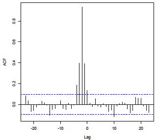
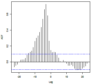
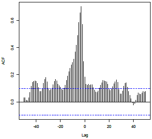
Following is the CCF of the simulated x and y series. We aren’t able to learn anything from it.
- Step 1
We determine a (possibly approximate) ARIMA model for the x-series. The usual steps would be used. In this case, the ACF of the x-series did not taper to 0 suggesting a non-stationary series. Thus a first difference should be tried. The ACF and PACF of the first differences showed the prototypical pattern of an AR(1), so an ARIMA(1,1,0) should be tried.
For the simulated data, the estimated phi-coefficient for the ARIMA(1,1,0) was \(\widehat{\phi}_1 = 0.7445\).
The estimated model can be written as \( \left(1 - 0.7445B \right) \left(1 - B \right)\left(x_t - \mu \right) = w_t\).
In this form, we’re applying the AR(1) polynomial and a first difference to the x-variable.
- Step 2
Filter the y series using the model for x.
We don’t need to worry about the mean because correlations aren’t affected by the level of the mean. Thus, we’ll calculate the filtered y as
\( \left(1 - 0.7445B \right) \left(1 - B \right) y_{t} = \left(1 - 1.7445B + 0.7445B^{2} \right)y_{t}\)
In the equation(s) just given, the AR(1) polynomial for x and the first differencing are applied to the y-series. An R command that carrys out this operation is:
newpwy = filter(y, filter = c(1,-1.7445,.7445), sides =1) - Step 3
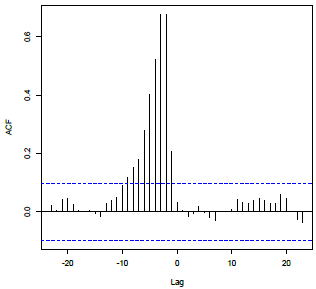
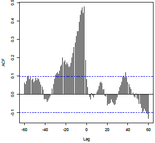
For the simulated data, the following plot is the CCF for the pre-whitened x and the filtered y. The pre-whitened x = residuals from ARIMA(1,1,0) for x. We see clear spikes at lags 3 and 4. Thus \(x_{t-3}\) and \(x_{t-4}\) should be tried as predictors of \(y_{t}\) .
R
R Code for the Example 9-1
Here’s the R Code for the example. The code includes all steps, including the simulation of the series, and the estimation of the lagged regression after identification of the model has been done. The filter command would have to be modified in a new simulation because the AR coefficient would be different for a new sample.
x = arima.sim(list(order = c(1,1,0), ar = 0.7), n = 200) #Generates random data from ARIMA(1,1,0). This will generate a new data set for each call.
z = ts.intersect(x, lag(x,-3), lag(x,-4)) #Creates a matrix z with columns, xt, xt-3, and xt-4
y = 15+0.8*z[,2]+1.5*z[,3] #Creates y from lags 3 and 4 of randomly generated x
ccf(z[,1],y,na.action = na.omit) #CCF between x and y

acf(x)
diff1x=diff(x,1)
acf(diff1x, na.action = na.omit)
pacf(diff1x, na.action = na.omit)
ar1model = sarima(x,1,1,0)
ar1model
pwx=resid(ar1model$fit)
newpwy = filter(y, filter = c(1,-1.7445,.7445), sides =1)
ccf (pwx,newpwy,na.action=na.omit)
Note!
na.action = na.omit ignores the missing values within the data set a created by aligning the rows of y with lags of x. Print a to see the missing values listed as NA.
If you use arima rather than sarima, you must use: pwx = ar1model$residuals to access the residuals.
CCF Patterns
In general, we’re trying to identify lags of x and y that might predict y. The following table describes some typical situations with a peak at lag d. Notice that a smooth tapering pattern in the CCF indicates that we should use \(y_{t-1}\) and perhaps even \(y_{t-2}\) along with lags of x.
| Pattern in CCF | Regression Terms in Model |
|---|---|
|
Non-zero values at lag d and perhaps other lags beyond d, with no particular pattern; correlations near 0 at other lags. Pattern 1 Example
Non-zero values at lag d and perhaps other lags beyond d, with no particular pattern; correlations near 0 at other lags. |
X: Lag d, \(x_{t-d}\) and perhaps additional lags of x Y: No lags of y |
|
Exponential decay of correlations beginning at lag d; correlations near 0 at lags before lag d. Pattern 2 Example
Exponential decay of correlations beginning at lag d; correlations near 0 at lags before lag d. |
X: Lag d, \(x_{t-d}\) Y: Lag 1, \(y_{t-1}\) |
|
Non-zero correlations with no particular pattern beginning at lag d, but then exponential decay begins at last used lag of x; correlations near 0 before lag d. Pattern 3 Example
Non-zero correlations with no particular pattern beginning at lag d, but then exponential decay begins at last used lag of x; correlations near 0 before lag d. |
X: Lag d, \(x_{t-d}\), and perhaps additional lags of x. Y: Lag 1, \(y_{t-1}\) |
|
Sinusoidal pattern beginning at lag d, with decay toward 0; correlations near 0 before lag d. Pattern 4 Example
Sinusoidal pattern beginning at lag d, with decay toward 0; correlations near 0 before lag d. |
X: Lag d, \(x_{t-d}\) Y: Lags 1 and 2, \(y_{t-1}\), \(y_{t-2}\) |
|
Non-zero correlations with no particular pattern beginning at lag d, but then Sinusoidal pattern beginning at last used lag of x, with decay toward 0; correlations near 0 before lag d. Pattern 5 Example
Non-zero correlations with no particular pattern beginning at lag d, but then Sinusoidal pattern beginning at lag d, with decay toward 0; correlations near 0 before lag d. |
X: Lag d, \(x_{t-d}\), and perhaps additional lags of x. Y: Lags 1 and 2, \(y_{t-1}\), \(y_{t-2}\) |
- Examine the CCF for the original data
- If it is unclear, determine a time series for x, and find the residuals
- Pre-whiten
- Examine the CCF for the pre-whitened x and the filtered y
Transfer Functions
The term “transfer function” applies to models in which we predict y from past lags of both y and x (including possibly lag 0), and we also model x and the errors. For prediction of the future past the end of the series, we might first use the model for x to forecast x. Then we would use the forecasted x when we forecast future y.
9.2 Intervention Analysis
9.2 Intervention AnalysisSuppose that at time \(t\) = T (where T will be known), there has been an intervention to a time series. By intervention, we mean a change to a procedure, or law, or policy, etc. that is intended to change the values of the series \(x_{t}\). We want to estimate how much the intervention has changed the series (if at all). For example, suppose that a region has instituted a new maximum speed limit on its highways and wants to learn how much the new limit has affected accident rates.
Intervention analysis in time series refers to the analysis of how the mean level of a series changes after an intervention, when it is assumed that the same ARIMA structure for the series \(x_{t}\) holds both before and after the intervention.
Overall Intervention Model
Suppose that the ARIMA model for \(x_{t}\) (the observed series) with no intervention is
\(x_t - \mu = \dfrac{\Theta(B)}{\Phi(B)}w_t\)
with the usual assumptions about the error series \(w_{t}\).
\(\Theta(B)\) is the usual MA polynomial and \(\Phi(B)\) is the usual AR polynomial.
Let \(z_{}\)= the amount of change at time \(t\) that is attributable to the intervention. By definition, \(z_{t}\) = 0 before time T (time of the intervention). The value of \(z_{t}\) may or may not be 0 after time T.
Then the overall model, including the intervention effect, may be written as
\(x_t - \mu = z_t + \dfrac{\Theta(B)}{\Phi(B)}w_t\)
Example 9-2
Following is a plot of a simulated MA(2) model with mean μ = 60 prior to an “intervention point” at time \(t\) = 100. We added 10 to the series for times \(t\) ≥ 100. In practice, the task would be to determine the magnitude and pattern of the change to the series.
Possible Patterns for Intervention Effect (patterns for \(z_t\))
There are several possible patterns for how an intervention may affect the values of a series for \(t\) ≥ T (the intervention point). Four possible patterns are as follows:
Permanent constant change to the mean level: An amount has been added (or subtracted) to each value after time T.
Brief constant change to the mean level: There may be a temporary change for one or more periods, after which there is no effect of the intervention.
Gradual increase or decrease to a new mean level: There may be a gradually increasing amount that is added (or subtracted) which eventually levels off at a new level (compared to the “before” level).
Initial change followed by gradual return to the no change: There may be an immediate change to the values of the series, but the amount added or subtracted to each value after time T approaches 0 over time.
Models for the Patterns
\(z_{t}\) = the amount of change at time \(t\) that is attributable to the intervention.
Suppose that \(I_{t}\) is an indicator variable such that \(I_{t}\) = 1 when \(t\) ≥ T and \(I_{t}\) = 0 when \(t\) < T.
- Pattern 1
Constant permanent change. A constant change of equal to the amount \(\delta_0\) after time T may be written simply as
\(z_{t}\) = \(\delta_0\)\(I_{t}\).
Note!\(z_{t}\) = \(\delta_0\) for \(t\) ≥ T, and \(z_{t}\) = 0 and for \(t\) < T. The coefficient \(\delta_0\) will be estimated using the data. - Pattern 2
A temporary (constant change) lasting for d times past the intervention time T, can be described by the intervention effect model
\(z_{t}\) = \(\delta_0 \left(1 - B^{d} \right) I_{t}\).
Or, we can redefine the indicator so that \(I_{t}\) = 1 for T ≤ \(t\) ≤ T + d, and \( I_{t} \) = 0 for all other \(t\). Then, we use the model \(z_{t}\) = \(\delta_0\)\(I_{t}\).
With this intervention effect, \(z_{t}\) = \(\delta_0\) for T ≤ \(t\) ≤ T + d, and \(z_{t}\) = 0 and for all other \(t\). Again, the coefficient \(\delta_0\) will be estimated using the data.
- Pattern 3
A gradually increasing effect that eventually levels off can be written as:
\(z_t = \dfrac{\delta_0}{1-\omega_1B}I_t,\)
with \(I_{t}\) = 1 for \(t\) ≥ T and \(I_{t}\) = 0 when \(t\) < T. Assume \(\lvert\omega_1\rvert\) < 1.
This is equivalent to \(z_{t}\) = \(\omega_1\)\(z_{t-1}\) + \(\delta_0\)\(I_{t}\).
When \(t\) < T, \(z_{t}\) = 0.
When \(t\) ≥ T, \(I_{t}\) =1 so \(z_{t}\) = \(\omega_1\)\(z_{t-1}\) + \(\delta_0\). Because \(\lvert\omega_1\rvert\) < 1, we can continue to express each past \(z_{t}\) in terms of \(\omega_1\) and \(\delta_0\) as a geometric series to obtain the following:
\(z_t = \dfrac{\delta_0 (1-\omega_1^{t-T+1})}{1-\omega_1}.\)
The coefficients \(\omega_1\) and \(\delta_0\) will be estimated using the data.
- Pattern 4
An immediate change that eventually returns to 0 can be modeled as follows
\(z_t = \dfrac{\delta_0}{1-\omega_1B}P_t ,\)
with \(P_{t}\) = 1 when t = T and \( P_{t} \) = 0 otherwise. Assume \( \lvert\omega_1\rvert\) < 1.
This is equivalent to \(z_{t}\) = \(\omega_1\)\(z_{t-1}\) + \(\delta_0 P_{t}\).
When \(t < T\), \(z_{t}\) = 0.
When \(t = T\), \(z_{t-1}\) = 0 and \(P_{t }\)= 1 so \(z_{t}\) = \(\delta_0\).
When \(t ≥ T+1\), \(P_{t }\)= 0 so \(z_{t}\) = \(\omega_1\)\(z_{t-1}\).
The coefficients \(\omega_1\) and \(\delta_0\) will be estimated using the data.
Estimating the Intervention Effect
Two parts of the overall model have to be estimated – the basic ARIMA model for the series and the intervention effect. Several approaches have been proposed. One approach has the following steps:
- Use the data before the intervention point to determine the ARIMA model for the series.
- Use that ARIMA model to forecast values for the period after the intervention.
- Calculate the differences between actual values after the intervention and the forecasted values.
- Examine the differences in step 3 to determine a model for the intervention effect.
What we do after step 4 depends on available software. If the right program is available we can use all of the data to estimate the overall model that combines the ARIMA for the series and the intervention model. Otherwise, we might use only the differences from step 4 above to make estimates of the magnitude and nature of the intervention.
Example 9-3
North Carolina Highway Fatality Rates, monthly for n = 86 months. Beginning at month = 71 the maximum speed limit was lowered from 70 mph to 55 mph. The fatality rate is computed as highway fatalities per 100 million miles of travel. A time series plot follows. The latter part of the series, in red, is the fatality rate after the change in speed limit.
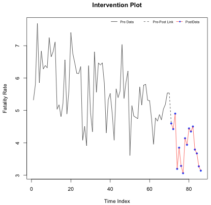
Using the data from times \(t\) = 1, …, 70 (before the speed limit decrease), we fit an ARIMA (2, 1, 0) × (1, 1, 0)12.
Coefficients:
ar1 ar2 sar1
-0.8142 -0.6461 -0.3717
s.e. 0.1081 0.1119 0.1278
sigma^2 estimated as 0.5834: log likelihood = -67.04, aic = 142.08
We then use this model to forecast values for \(t\) = 71, …, 86 and compare the forecasted values to the actual values during this intervention period. The first of the next two plots shows the forecasted values compared to the actual values for the “after” period. The second plot shows the differences.
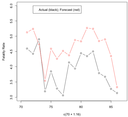
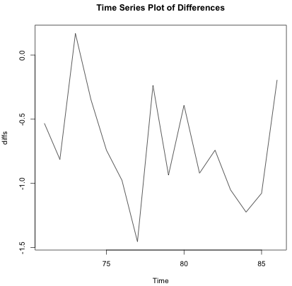
It’s difficult to judge the mean intervention pattern exactly. It’s possible that a constant mean change may describe the situation. The mean difference between actual and forecasted in the intervention period is -0.7168515.
We’ll learn how to do things in R in the homework for this week.