8.1 Linear Regression Models with Autoregressive Errors
8.1 Linear Regression Models with Autoregressive ErrorsWhen we do regressions using time series variables, it is common for the errors (residuals) to have a time series structure. This violates the usual assumption of independent errors made in ordinary least squares regression. The consequence is that the estimates of coefficients and their standard errors will be wrong if the time series structure of the errors is ignored.
It is possible, though, to adjust estimated regression coefficients and standard errors when the errors have an AR structure. More generally, we will be able to make adjustments when the errors have a general ARIMA structure.
The Regression Model with AR Errors
Suppose that yt and xt are time series variables. A simple linear regression model with autoregressive errors can be written as
\(y_{t} =\beta_{0}+\beta_{1}x_{t}+\epsilon_{t}\)
with \(\epsilon_t = \phi_{1}\epsilon_{t-1}+\phi_{2}\epsilon_{t-2}+ \cdots + w_t\), and \(w_t \sim \text{iid}\; N(0, \sigma^2)\).
If we let \(\Phi(B)=1-\phi_{1}B- \phi_{2}B^2 - \cdots\), then we can write the AR model for the errors as
\(\Phi(B)\epsilon_{t}=w_{t}.\)
If we assume that an inverse operator, \(\Phi^{-1}(B)\), exists, then \(\epsilon_{t}=\Phi^{-1}(B)w_{t}\).
So, the model can be written
\(y_t =\beta_{0} +\beta_{1}x_{t} + \Phi^{-1}(B)w_{t},\)
where \(w_{t}\) is the usual white noise series.
This generalizes to the multiple linear regression structure as well. We can have more than one x-variable (time series) on the right side of the equation. Each x-variable is adjusted in the manner described below.
Examining Whether This Model May be Necessary
- Start by doing an ordinary regression. Store the residuals.
- Analyze the time series structure of the residuals to determine if they have an AR structure.
- If the residuals from the ordinary regression appear to have an AR structure, estimate this model and diagnose whether the model is appropriate.
Theory for the Cochrane-Orcutt Procedure
A simple regression model with AR errors can be written as
\((1) \;\;\; y_t =\beta_0 +\beta_1x_t + \Phi^{-1}(B)w_{t}\)
\(\Phi(B)\) gives the AR polynomial for the errors.
If we multiply all elements of the equation by \(\Phi(B)\), we get
\(\Phi(B)y_t = \Phi(B)\beta_0 +\beta_1\Phi(B)x_t + w_t\)
- Let \(y^{*}_{t} =\Phi(B)y_{t} = y_{t} - \phi_{1}y_{t-1} - \cdots - \phi_{p}y_{t-p}\)
- Let \(x^{*}_{t} =\Phi(B)x_{t} = x_{t} - \phi_{1}x_{t-1} - \cdots - \phi_{p}x_{t-p}\)
- Let \(\beta^{*}_{0} =\Phi(B)\beta_{0} = (1 - \phi_{1} - \cdots - \phi_{p})\beta_{0}\)
In the last of the equations just given \(\beta_{0}\) is an unknown constant that does not move in time. Thus it is not affected by any backshift operation. That’s why the B operations were not applied in that equation.
Using the items just defined, we can write the model as
\((2) \;\;\; y^*_t =\beta^*_0 +\beta_1x^*_t + w_{t}\)
Remember that \(w_t\) is a white noise series, so this is just the usual simple regression model.
We use results from model (2) to iteratively adjust our estimates of coefficients in model (1).
- The estimated slope \(\widehat{\beta}_1\) from model (2) will be the adjusted estimate of the slope in model (1) (and its standard error from this model will be correct as well).
- To adjust our estimate of the intercept \(\beta_0\) in model (1), we use the relationship \(\beta^*_0=(1 - \phi_{1} - \cdots - \phi_{p})\beta_{0}\) to determine that
\(\widehat{\beta}_0=\dfrac{\widehat{\beta}^*_0}{1 - \widehat{\phi}_{1} - \cdots - \widehat{\phi}_{p}}.\)
The standard error for \(\widehat{\beta}_0\) is\(s.e.( \widehat{\beta}_0) =\dfrac {s.e. ( \widehat{\beta}^{*}_{0})} {1 - \widehat{\phi}_{1} - \cdots - \widehat{\phi}_{p}}.\)
This procedure is attributed to Cochrane and Orcutt (1949) and is repeated until the estimates converge, that is we observe a very small difference in our estimates between iterations. When the errors exhibit an AR(1) pattern, the cochrane.orcutt function found within the orcutt package in R iterates this procedure.
Additional Comment
For a higher order AR, the adjustment variables are calculated in the same manner with more lags. For instance, suppose the residuals were found to have an AR(2) with estimated coefficients 0.9 and -0.2. Then the y- and x- variables for the adjustment regression would be
\(y^{*}_{t} = y_{t} - 0.9y_{t-1}+0.2y_{t-2}\)
\(x^{*}_{t} = x_{t} - 0.9x_{t-1}+0.2x_{t-2}\)
Example 8-1: Economic Measure
There are n = 76 annual observations in sequence. Suppose x is a leading economic indicator (predictor) for a country and y = a measure of the state of the economy. The following plot shows the relationship between x and y for 76 years.

Suppose that we want to estimate the linear regression relationship between y and x at concurrent times.
- Step 1
Estimate the usual regression model. Results from R are:
Coefficients: Estimate Std. Error t value Pr(>|t|) (Intercept) 3.600e+04 7.152e+01 503.373 < 2e-16 *** x 1.610e+00 2.023e-01 7.956 1.57e-11 *** (It is not shown, but worthy to note that trend=time(x) is not significant in this regression and x is not changing over time.)
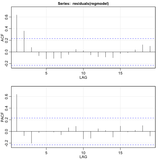
- Step 2
Examine the AR structure of the residuals. Following are the ACF and PACF of the residuals. It looks like the errors from Step 1 have an AR(1) structure.
- Step 3
Estimate the AR coefficients (and make sure that the AR model actually fits the residuals). For this example, the R estimate of the AR(1) coefficient is:
Coefficients: ar1 0.6488 s.e. 0.0875 Model diagnostics (not shown here) were okay.
- Step 4
Calculate variables to use in the adjustment regression:
\(x^*_t = x_t - 0.6488x_{t-1}\)
\(y^*_t = y_t - 0.6488y_{t-1}\)
- Step 5
Use ordinary regression to estimate the model \(y^*_t = \beta^*_0 + \beta_1 x^*_t +w_t\). For this example, the results are
Coefficients: Estimate Std. Error t value Pr(>|t|) (Intercept) 1.264e+04 1.476e+01 856.50 < 2e-16 *** xnew 1.635e+00 1.174e-01 13.93 < 2e-16 *** The slope estimate (1.64) and its standard error (0.1174) are the adjusted estimates for the original model.
The adjusted estimate of the intercept of the original model is 12640/(1-0.6488) = 35990. The estimated standard error of the intercept is 14.76/(1-0.6488) = 42.03.
This procedure is iterated until the estimates converge. In R, the Cochrane.orcutt function iterates the steps:
Coefficients: Estimate Std. Error t value Pr(>|t|) (Intercept) 3.5995e+04 4.2215e+01 852.650 < 2.2e-16 *** x 1.6347e+00 1.1805e-01 13.848 < 2.2e-16 *** Signif. codes: 0 ‘***’ 0.001 ‘**’ 0.01 ‘*’ 0.05 ‘.’ 0.1 ‘ ’ 1
Residual standard error: 19.5133 on 73 degrees of freedom
Multiple R-squared: 0.7243, Adjusted R-squared: 0.7205
F-statistic: 191.8 on 1 and 73 DF, p-value: < 4.106e-22$rho
[1] 0.638412$number.interaction
[1] 4The slope estimate (1.635) and its standard error (0.11805) are the adjusted estimates for the original model.
Thus our estimated relationship between \(y_t\) and \(x_t\) is
\(y_t = 35995 + 1.635x_t\)
The errors have the estimated relationship \(e_t = 0.6384 e_{t-1} + w_t\).
Note!The predicted y is a linear function of x at this time and the residual at the previous time.
R
The R Program
Download the data used in the following code: econpredictor.dat , econmeasure.dat
x=ts(scan("econpredictor.dat"))
y=ts(scan("econmeasure.dat"))
plot.ts(x,y,xy.lines=F,xy.labels=F)

regmodel=lm(y~x)
summary(regmodel)
acf2(residuals(regmodel))

ar1res = sarima (residuals(regmodel), 1,0,0, no.constant=T) #AR(1)
xl = ts.intersect(x, lag(x,-1)) # Create matrix with x and lag 1 x as elements
xnew=xl[,1] - 0.6488*xl[,2] # Create x variable for adjustment regression
yl = ts.intersect(y,lag(y,-1)) # Create matrix with y and lag 1 y as elements
ynew=yl[,1]-0.6488*yl[,2] # Create y variable for adjustment regression

adjustreg = lm(ynew~xnew) # Adjustment regression
summary(adjustreg)
acf2(residuals(adjustreg))

install.packages("orcutt")
library(orcutt)
cochrane.orcutt(regmodel)
summary(cochrane.orcutt(regmodel))
A potential problem with the Cohrane-Orcutt procedure is that the residual sum of squares is not always minimized and therefore we now present a more modern approach following our text.
The Regression Model with ARIMA Errors
Estimating the Coefficients of the Adjusted Regression Model with Maximum Likelihood
The method used here depends upon what program you're using. In R (with gls and arima) and in SAS (with PROC AUTOREG) it's possible to specify a regression model with errors that have an ARIMA structure. With a package that includes regression and basic time series procedures, it's relatively easy to use an iterative procedure to determine adjusted regression coefficient estimates and their standard errors. Remember, the purpose is to adjust "ordinary" regression estimates for the fact that the residuals have an ARIMA structure.
Carrying out the Procedure
The basic steps are:
- Step 1
Use ordinary least squares regression to estimate the model \(y_t =\beta_0 +\beta_1t + \beta_2x_t + \epsilon_t\)
Note!We are modeling a potential trend over time with \(\beta_0 + \beta_1t\) and may need to de-trend x if x is strongly correlated with time, \(t\). Please see Section 2.2 of the text for a discussion on de-trending. - Step 2
Examine the ARIMA structure (if any) of the sample residuals from the model in step 1.
- Step 3
If the residuals do have an ARIMA structure, use maximum likelihood to simultaneously estimate the regression model using ARIMA estimation for the residuals.
- Step 4
Examine the ARIMA structure (if any) of the sample residuals from the model in step 3. If white noise is present, then the model is complete. If not, continue to adjust the ARIMA model for the errors until the residuals are white noise.
Example 8-2: Simulated
The following plot shows the relationship between a simulated predictor x and response y for 100 annual observations.

Suppose that we want to estimate the linear regression relationship between y and x at concurrent times.
- Step 1: Estimate the usual regression model.
Results from R are:
Coefficients: Estimate Std. Error t value Pr(>|t|) (Intercept) 57.76368 3.84725 15.014 < 2e-16 *** trend 0.03450 0.09416 0.366 0.715 x 0.41798 0.18859 2.216 0.029 * Residual standard error: 1.774 on 97 degrees of freedom
Multiple R-squared: 0.9416, Adjusted R-squared: 0.9404
F-statistic: 782.1 on 2 and 97 DF, p-value: < 2.2e-16Trend is not significant, however we notice that x is increasing over time as well and is strongly correlated with time, r = .998. To reduce the multicollinearity between x and t, we can detrend x and examine the regression for y on the de-trended x, dtx, and time, t. The regression results are now:
Coefficients: Estimate Std. Error t value Pr(>|t|) (Intercept) 66.253549 0.357552 185.298 < 2e-16 *** trend 0.242735 0.006147 39.489 < 2e-16 *** dtx 0.417980 0.188592 2.216 0.029 * Residual standard error: 1.774 on 97 degrees of freedom
Multiple R-squared: 0.9416, Adjusted R-squared: 0.9404
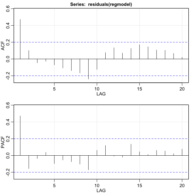
F-statistic: 782.1 on 2 and 97 DF, p-value: < 2.2e-16 - Step 2: Examine the ARIMA structure of the residuals.
Following are the ACF and PACF of the residuals. Because both the ACF and PACF spike and then cut off, we should compare AR(1), MA(1), and ARIMA(1,0,1). We will continue with the MA(1) model in the notes.
- Step 3: Estimate the adjusted model with a MA(1) structure for the residuals (and make sure that the MA model actually fits the residuals)
For this example, the R estimate of the model is
Coefficients: ma1 intercept trend dtx 0.4551 66.2633 0.2423 0.4364 s.e. 0.0753 0.4489 0.0077 0.1421 sigma^2 estimated as 2.380735 on 96 degrees of freedom
AIC = 3.807608 AICc = 3.811818 BIC = 3.937866 - Step 4: Model diagnostics, (not shown here), suggested that the model fit well.
Thus our estimated relationship between \(y_t\) and \(x_t\) is
\(y_t = 66.26 + 0.24t + 0.44dtx_t + e_t \)
The errors have the estimated relationship \(e_t = w_t + 0.46w_{t−1}\) , where \(w_t \sim \text{iid} \; N(0,\sigma^2)\).
R
The R Program
The data are in two files: l8.1x.dat and l8.1y.dat.
library(astsa)
x=ts(scan("l8.1.x.dat"))
y=ts(scan("l8.1.y.dat"))
plot(x,y, pch=20,main = "X versus Y")

trend = time(y)
regmodel=lm(y~trend+x) # first ordinary regression.
dtx = residuals(lm (x~time(x)))
regmodel= lm(y~trend+dtx) # first ordinary regression with detrended x, dtx.
summary(regmodel) # This gives us the regression results
acf2(resid(regmodel)) # ACF and PACF of the residuals

adjreg = sarima (y, 0,0,1, xreg=cbind(trend, dtx)) # This is the adjustment regression with MA(1) residuals
adjreg # Results of adjustment regression. White noise should be suggested.
acf2(resid(adjreg$fit))

library(nlme)
summary(gls(y ~ dtx+trend, correlation = corARMA(form = ~ 1,p=0,q=1))) #For comparison
Example 8-3: Glacial Varve
Note that in this example it might work better to use an ARIMA model as we have a univariate time series, but we’ll use the approach of these notes for illustrative purposes. We analyze the glacial varve data described in Example 2.5, page 62 of the text. The response is a measure of the thickness of deposits of sand and silt (varve) left by spring melting of glaciers about 11,800 years ago. The data are annual estimates of varve thickness at a location in Massachusetts for 455 years beginning 11,834 years ago. There are nonconstant variance and outlier problems in the data, so we might try a log transformation with hopes of stabilizing the variance and diminishing the effects of outliers. Here’s a time series plot of the log10 series.
There’s a curvilinear pattern, so we’ll try the ordinary regression model
\( \text{log}_{10} y = \beta_0 + \beta_1 (t-\bar{t}) + \beta_2(t-\bar{t})^2 + \epsilon\),
where \(t\) = year numbered 1, 2, …455.
Centering the time variable creates uncorrelated estimates of the linear and quadratic terms in the model. Regression results found using R are:
| Estimate | Std. Error | t value | Pr(>|t|) | |
|---|---|---|---|---|
| (Intercept) | 1.220e+00 | 1.502e-02 | 81.19 | < 2e-16 *** |
| trend | 9.047e-04 | 7.626e-05 | 11.86 | < 2e-16 *** |
| trend2 | 8.283e-06 | 6.491e-07 | 12.76 | < 2e-16 *** |
Residual standard error: 0.2137 on 452 degrees of freedom
Multiple R-squared: 0.4018, Adjusted R-squared: 0.3991
F-statistic: 151.8 on 2 and 452 DF, p-value: < 2.2e-16
The autocorrelation and partial autocorrelation functions of the residuals from this model follow.
Similar to example 1, we might interpret the patterns either as an ARIMA(1,0,1), an AR(1), or a MA(1). We’ll pick the AR(1) – in large part to show an alternative to the MA(1) in Example 2.
The ARIMA results for a AR(1):
| ar1 | intercept | trend | trend2 | |
|---|---|---|---|---|
| 0.2810 | 1.2200 | 9e-04 | 8e-06 | |
| s.e. | 0.0466 | 0.0202 | 1e-04 | 4e-05 |
sigma^2 estimated as 0.04176: log likelihood = 76.86, aic = -143.72
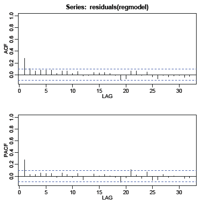
Check diagnostics:
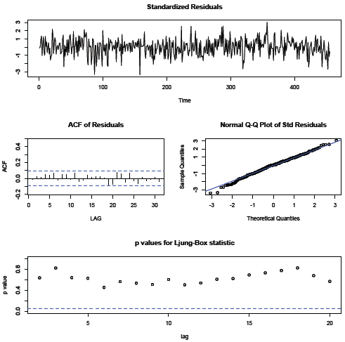
The autocorrelation and partial autocorrelation functions of the residuals from this estimated model include no significant values. The fit seems is satisfactory, so we’ll use these results as our final model. The estimated model is
\(\text{log}_{10}y =1.22018 + 0.0009029(t − \bar{t}) + 0.00000826(t − \bar{t})^2,\)
with errors \(e_t = 0.2810 e_{t-1} +w_t\) and \(w_t \sim \text{iid} \; N(0,\sigma^2)\).
The predicted y is a linear function of time and the residual at the previous time.
R
The R Program
The data are in varve.dat in the Week 8 folder, so you can reproduce this analysis or compare to a MA(1) for the residuals.
library(astsa)
varve=scan("varve.dat")
varve=ts(varve[1:455])
lvarve=log(varve,10)
trend = time(lvarve)-mean(time(lvarve))
trend2=trend^2
regmodel=lm(lvarve~trend+trend2) # first ordinary regression.
summary(regmodel)
acf2(resid(regmodel))
adjreg = sarima (lvarve, 1,0,0, xreg=cbind(trend,trend2)) #AR(1) for residuals
adjreg #Note that the squared trend is not significant, but should be kept for diagnostic purposes.
adjreg$fit$coef #Note that R actually prints 0’s for trend2 because the estimates are so small. This command prints the actual values.