13.1 Long Memory Models and Fractional Differences
13.1 Long Memory Models and Fractional DifferencesSection 5.1 of Shumway and Stoffer gives a brief overview of “long memory ARMA” models. This type of model may possibly be used when the ACF of the series tapers slowly to 0.
The usual solution in this situation is to explore the first differences of the series. Often, data for which a first difference is successful will typically have a first lag autocorrelation quite close to 1.
A model for a first difference could be written in the format
\(x_t - x_{t-1}\) = AR and MA terms.
This can be rewritten as
\(x_t = x_{t-1} +\) AR and MA terms.
In this formulation we have a first lag AR type of term with a coefficient equal to 1. This creates a first order autocorrelation for the original series close to 1.
In some instances, however, we may see a persistent pattern of non-zero correlations that begins with a first lag correlation that is not close to 1. In these cases, models that incorporate “fractional differencing” may be useful. A simple model that utilizes fractional differencing is
\((1-B)^dx_t = w_t\)
where d is a value such that |d| < .5 and wt is the usual white noise term.
Mathematically, this model can be expanded to be an infinite order AR with coefficients that may taper (very) slowly toward 0. We’ll skip those details (the results are given on pages 268-269 of our text).
In a fractionally differenced model, the difference coefficient d is a parameter to be estimated. The R package arfima can be used to do this. Again, an indication that this model might be useful is a slowly tapering sample ACF without particularly high autocorrelations.
Example 5.1 in the text looks at a fractionally differenced model for a series of n = 634 (yearly) values of a geological measurement called varve. This is a sedimentary layer of sand and silt left by melting glaciers. A time series plot of the data follows.
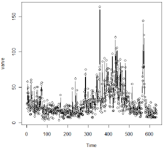
Due to the period of more extreme variability, the authors suggest analyzing the logarithm of the data. (This might stabilize the variance.)
A plot of the log-transformed series follows:
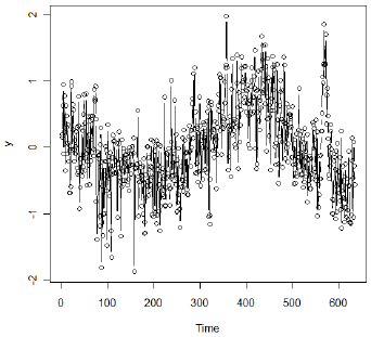
The sample ACF of the log-transformed data shows a persistent pattern of moderately high values. Here’s both the ACF and the PACF. In Chapter 3 of the text the authors use first differencing and explore the relative merits of ARIMA(0,1,1) and ARIMA(1,1,1) models for these data. In Section 5.1, the authors explore a fractionally differenced model.
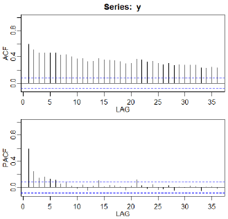
The arfima package gives an estimate for the differencing fraction of \(\widehat{d} = 0.373\). Thus the estimated model is \((1-B)^{.373}x_t = w_t\) where \(x_t\) is the centered log-transformed log series.
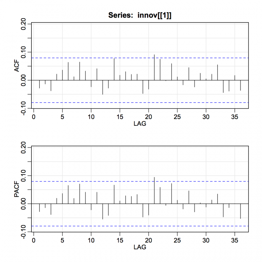
This model provides a good fit to the data as evidenced by the following ACF and PACF of the residuals.
Generalizations
The model can be expanded to include AR and MA terms as well as the fractional difference. These models are called ARFIMA models. To identify an ARFIMA model, we first use the simple fractional difference model \((1-B)^dx_t = w_t\) and then explore the ACF and PACF of the residuals from this model. This is analogous to exploring the ACF and PACF of the first differences when we carry out the usual steps for non-stationary data. The arfima package can be used to fit general ARFIMA models.
Interpretation Difficulty
The main difficulty is that a fractional difference is difficult to interpret. Basically it’s a mathematical device that is used to expand a model into a high order AR with autocorrelations that match the persistent ”long memory” pattern of the ACF of the series.
R R Code for Example 5.1
For the following code to run, you have to install the arfima package; this is strongly encouraged over the fracdiff package covered in the text (http://www.stat.pitt.edu/stoffer/tsa4/Rexamples.htm). Once the package is installed on your system, you can skip the installation step and use library(arfima) just as we have for the astsa library.
varve = scan("varve.dat")
varve = ts(varve)
library(astsa)
install.packages("arfima")
library(arfima)

y = log(varve) - mean(log(varve)) # Center the logs
acf2(y) ## ACF and PACF of the data

## Estimate d:
varvefd = arfima(y)
summary(varvefd)
d = summary(varvefd)$coef[[1]][1]   #d = 0.3727
d   #prints the value of d to the screen
se.d = summary(varvefd)$coef[[1]][1,2]   #se = 0.0273
se.d   #prints the standard error of d to the screen


##Residuals

resids = resid(varvefd)[[1]]
#resid(varvefd) is a list and [[1]] accesses the residuals as a vector
plot.ts(resids)
acf2(resids)