| Key Learning Goals for this Lesson: |
Textbook reading: Consult Course Schedule |
Principal Component Analysis (PCA) is a method of dimension reduction. This is not directly related to prediction problem, but several regression methods are directly dependant on it. The regression methods (PCR and PLS) will be considered later. Now a motivation for dimension reduction is being set up.
The input matrix X of dimension \(N \times p\):
\[\begin{pmatrix}
x_{1,1} & x_{1,2} & ... & x_{1,p} \\
x_{2,1} & x_{2,2} & ... & x_{2,p}\\
... & ... & ... & ...\\
x_{N,1} & x_{N,2} & ... & x_{N,p}
\end{pmatrix}\]
The rows of the above matrix represent the cases or observations.
The columns represent the variables observed on each unit. These represent the characteristics.
Assume that the columns of X are centered, i.e., the estimated column mean is subtracted from each column.
Singular value decomposition is the key part of principal components analysis.
The SVD of the \(N × p\) matrix \(\mathbf{X}\) has the form \(\mathbf{X} = \mathbf{U}\mathbf{D}\mathbf{V}^T\).
The columns of \(\mathbf{V}\) (i.e., \(\mathbf{v}_j, j = 1, \cdots , p)\) are the eigenvectors of \(\mathbf{X}^T\mathbf{X}\). They are called principal component direction of \(\mathbf{X}\).
The diagonal values in \(\mathbf{D}\) (i.e., \(\mathbf{d}_j, j = 1, \cdots , p)\) are the square roots of the eigenvalues of \(\mathbf{X}^T\mathbf{X}\).
The two-dimensional plane can be shown to be spanned by
It can be extended to the k-dimensional projection. We can take the process further, seeking additional linear combinations that maximize the variance subject to being uncorrelated with all those already selected.
Principal components analysis is one of the most common methods used for linear dimension reduction. The motivation behind dimension reduction is that, the process gets unweildy with a large number of variables while the large number does not add any new information to the process. An analogy may be drawn with variance inflation factors in multiple regression. If VIF corresponding to any predictor is large, that predictor is not included in the model, as that variable does not contribute any new information. On the other hand, because of linear dependence, the regression matrix may become singular. In a multivariate situation, it may well happen that, a few (or a large number of) variables have high interdependence. A linear combination of variables is then considered which are orthogonal to one another, but the total variability within the sample is preserved as much as possible.
Suppose the data is 10-dimensional but needs to be reduced to 2-dimensional. The idea of principal component analysis is to use two directions that capture the variation in the data as much as possible.
[Keep in mind that the dimensions to which data needs to be reduced, is usually not pre-fixed. After taking a look at the total proportion of variability captured, the reduction in dimension is determined. Here reduction of 10-dimensional space to 2-diemnsion space is for illustration only]
The sample covariance matrix of X is given as:
\[ S=\textrm{X}^T\textrm{X} /N \].
If you do the Eigen decomposition of \(X^TX\):
\[\begin{align*}\textrm{X}^T\textrm{X}
&= (\textrm{U}\textrm{D}\textrm{V}^T)^T(\textrm{U}\textrm{D}\textrm{V}^T)\\
&= \textrm{V}\textrm{D}^T\textrm{U}^T\textrm{U}\textrm{D}\textrm{V}^T\\
&=\textrm{V}\textrm{D}^2\textrm{V}^T
\end{align*}\]
It turns out that if you have done the singular value decomposition then you already have the Eigen value decomposition for \(X^TX\).
The \(D^2\) is the diagonal part of matrix D with every element on the diagonal squared.
Also, we should point out that we can show using linear algebra that \(X^TX\) is a semi-positive definite matrix. This means that all of the eigenvalues are guaranteed to be nonnegative. The eigen values are in matrix \(D^2\). Since these values are squared, every diagonal element is non-negative.
The eigenvectors of \(X^TX\), \(v_j\), can be obtained either by doing an Eigen decomposition of \(X^TX\), or by doing a singular value decomposition from X. These vj's are called principal component directions of X. If you project X onto the principal components directions you get the principal components.
\( \textrm{z}_1=\begin{pmatrix}
X_{1,1}v_{1,1}+X_{1,2}v_{1,2}+ ... +X_{1,p}v_{1,p}\\
X_{2,1}v_{1,1}+X_{2,2}v_{1,2}+ ... +X_{2,p}v_{1,p}\\
\vdots\\
X_{N,1}v_{1,1}+X_{N,2}v_{1,2}+ ... +X_{N,p}v_{1,p}\end{pmatrix}\)
\[Var(\textrm{z}_1)=d_{1}^{2}/N\]
![]() [1]
[1]
Why are we interested in this? Consider an extreme case, (lower right), where your data all lie in one direction. Although two features represent the data, we can reduce the dimension of the dataset to one using a single linear combination of the features (as given by the first principal component).
Just to summarize the way you do dimension reduction. First you have X, and you remove the means. On X you do a singular value decomposition and obtain matrices U, D, and V. Then you call every column vector in V, \(v_j\), where j = 1, ... , p. This vj is called the principal components direction. Let's say your original dimension is 10 and we wish to reduce this to 2 dimensions, what would we do? We would take \(v_1\) and \(v_2\) and project X to \(v_1\) and X to \(v_2\). To project, multiply X by \(v_1\) for a column vector of size N. X times \(v_2\) gives you another column vector of size N. These two column vectors reduce the dimensions so you have:
\[\begin{pmatrix}
\tilde{x}_{1,1} & \rightarrow & \tilde{x}_{1,v} \\
\tilde{x}_{2,1} & \rightarrow & \tilde{x}_{1,v} \\
\downarrow & & \downarrow\\
\tilde{x}_{N,1} & \rightarrow & \tilde{x}_{N,v}
\end{pmatrix}\]
Every row would be a reduced version of your original data. If I asked you to give me the 2 dimensional version of the second sample point, then you would you would look at the row highlighted below:
Capture the intrinsic variability in the data.
Reduce the dimensionality of a data set, either to ease interpretation or as a way to avoid overfitting and to prepare for subsequent analysis.
The sample covariance matrix of \(\mathbf{X}\) is \(\mathbf{S} = \mathbf{X}^T\mathbf{X}/\mathbf{N}\), since \(\mathbf{X}\) has zero mean.
Eigen decomposition of \(\mathbf{X}^T\mathbf{X}\):
\[\mathbf{X}^T\mathbf{X} = (\mathbf{U}\mathbf{D}\mathbf{V}^T)^T (\mathbf{U}\mathbf{D}\mathbf{V}^T) =\mathbf{V}\mathbf{D}^T\mathbf{U}^T\mathbf{U}\mathbf{D}\mathbf{V}^T = \mathbf{V}\mathbf{D}^2\mathbf{V}^T\]
The eigenvectors of \(\mathbf{X}^T\mathbf{X}\) (i.e., vj, j = 1, …, p) are called principal component directions of \(\mathbf{X}\).
The first principal component direction \(\mathbf{v}_1\) has the following properties that
The second principal component direction v2 (the direction orthogonal to the first component that has the largest projected variance) is the eigenvector corresponding to the second largest eigenvalue, \(\mathbf{d}_2^2\) , of \(\mathbf{X}^T\mathbf{X}\), and so on. (The eigenvector for the kth largest eigenvalue corresponds to the kth principal component direction \(\mathbf{v}_k\).)
The kth principal component of \(\mathbf{X}\), \(\mathbf{z}_k\), has maximum variance \(\mathbf{d}_1^2 / N\), subject to being orthogonal to the earlier ones.
Principal components analysis (PCA) projects the data along the directions where the data varies the most.
 The first direction is decided by \(\mathbf{v}_1\) corresponding to the largest eigenvalue \(d_1^2\).
The second direction is decided by \(\mathbf{v}_2\) corresponding to the second largest eigenvalue \(d_2^2\).
The variance of the data along the principal component directions is associated with the magnitude of the eigenvalues.
Scree Plot – This is a useful visual aid which shows the amount of variance explained by each consecutive eigenvalue.
The choice of how many components to extract is fairly arbitrary.
When conducting principal components analysis prior to further analyses, it is risky to choose too small a number of components, which may fail to explain enough of the variability in the data.
Diabetes data
The diabetes data set is taken from the UCI machine learning database repository at: https://archive.ics.uci.edu/ml/datasets/Pima+Indians+Diabetes [2].
Load data into R as follows:
# set the working directory
setwd("C:/STAT 897D data mining")
# comma delimited data and no header for each variable
RawData <- read.table("diabetes.data",sep = ",",header=FALSE)
In RawData, the response variable is its last column; and the remaining columns are the predictor variables.
responseY <- RawData[,dim(RawData)[2]]
predictorX <- RawData[,1:(dim(RawData)[2]-1)]
Principal component analysis is done by the princomp function. For computing the principal components, sometimes it is recommended the data be scaled first. However, one needs to judge whether scaling is necessary on a case by case base. For scaling, we can set the cor=T argument.
pca <- princomp(predictorX, cor=T) # principal components analysis using correlation matrix
$scores gives the principal components arranged in decreasing order of the standard deviations of the principal components. Suppose we want to get the first and second principal components. We use the following code. The scatter plot for the two components is then drawn.
pc.comp <- pca$scores
pc.comp1 <- -1*pc.comp[,1] # principal component 1 scores (negated for convenience)
pc.comp2 <- -1*pc.comp[,2] # principal component 2 scores (negated for convenience)
plot(pc.comp1, pc.comp2, xlim=c(-6,6), ylim=c(-3,4), type="n")
points(pc.comp1[responseY==0], pc.comp2[responseY==0], cex=0.5, col="blue")
points(pc.comp1[responseY==1], pc.comp2[responseY==1], cex=0.5, col="red")
The scattor plot of the first two principal components are shown in the following figure. The red circles show data in Class 1 (cases with diabetes), and the blue circles show Class 0 (non diabetes).
Figure 1: The scatter plot of the first two principal components for the Diabetes data
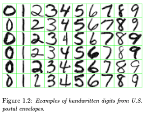
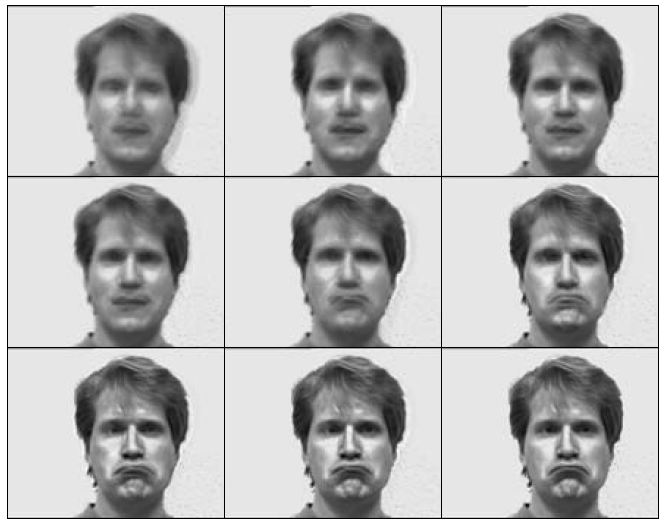
PCA can help you to transform the high dimension image data into lower dimension principal components.
The cumulative eff ect of nine principal components, adding one PC at a time, for "sad". The more principal components we use the better resolution we get. However, 4 or 5 principal components lead to a good judgement on a sad expression. It is a dramatic dimension reduction considering the original number of variables which is the number of pixels for a figure.
Why do dimensionality reduction?
When faced with situations involving high-dimensional data, it is natural to consider projecting those data onto a lower-dimensional subspace without losing important information.
Please finish the quiz for this lesson and the team project on ANGEL (check the course schedule for due dates).
Links:
[1] javascript:popup_window( 'https://www.youtube.com/embed/RcEbyFkIEJs?rel=0', 'pca_graph', 560, 315 );
[2] https://archive.ics.uci.edu/ml/datasets/Pima+Indians+Diabetes