Diabetes data
The diabetes data set is taken from the UCI machine learning database repository at: https://archive.ics.uci.edu/ml/datasets/Pima+Indians+Diabetes [1].
Load data into R as follows:
# set the working directory
setwd("C:/STAT 897D data mining")
# comma delimited data and no header for each variable
RawData <- read.table("diabetes.data",sep = ",",header=FALSE)
In RawData, the response variable is its last column; and the remaining columns are the predictor variables.
responseY <- as.matrix(RawData[,dim(RawData)[2]])
predictorX <- as.matrix(RawData[,1:(dim(RawData)[2]-1)])
For the convenience of visualization, we take the first two principal components as the new feature variables and conduct a logistic regression analysis only on these two dimensional data.
In R, glm performs the logistic regression analysis, and ()$fitted.values stores the fitted values for the response variable.
model.logistic <- glm(responseY~pc.comp1+pc.comp2, family=binomial("logit"))
In the case of binary classification, based on the fitted values of the response variable, we classify the sample point as Class 1 if its fitted value is greater than 0.5, otherwise Class 0. The scatter plot in Figure 1 shows the classification by the Logistic regression analysis. The red circles are Class 1 (with diabetes), and the blue circles are Class 0 (non diabetes).
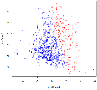
Figure 1: The classification result by logistic regression
Links:
[1] https://archive.ics.uci.edu/ml/datasets/Pima+Indians+Diabetes