Diabetes data
The diabetes data set is taken from the UCI machine learning database repository at: https://archive.ics.uci.edu/ml/datasets/Pima+Indians+Diabetes [1].
Load data into R as follows:
# set the working directory
setwd("C:/STAT 897D data mining")
# comma delimited data and no header for each variable
RawData <- read.table("diabetes.data",sep = ",",header=FALSE)
In RawData, the response variable is its last column; and the remaining columns are the predictor variables.
responseY <- as.matrix(RawData[,dim(RawData)[2]])
predictorX <- as.matrix(RawData[,1:(dim(RawData)[2]-1)])
For the convenience of visualization, we take the first two principle components as the new feature variables and conduct k-means only on these two dimensional data.
The MASS package contains functions for performing linear and quadratic discriminant analysis. Both estimate the class prior probabilities by the proportion of data in each class, unless prior probabilities are specified. The code below performs LDA.
library(MASS)
model.lda <- lda(responseY ~ pc.comp1+pc.comp2)
predict()$class predicts a class label for a new sample point using an obtained model, e.g., LDA model.
predict(model.lda)$class
The classification result by LDA is shown in Figure 1. The red circles correspond to Class 1 (with diabetes), the blue circles to Class 0 (non-diabetes).
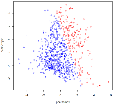
Figure 1: Classification result by LDA
Quadratic discriminant analysis does not assume homogeneity of the covariance matrices of all the class. The following code performs the QDA.
model.qda <- qda(responseY ~ pc.comp1+pc.comp2)
Again, we can use predict()$class to obtain classification result based on the estimated QDA model.
predict(model.qda)$class
The classification result by QDA is shown in Figure 2.
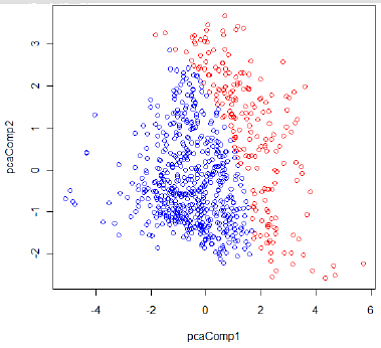
Figure 2: Classification result by QDA
Links:
[1] https://archive.ics.uci.edu/ml/datasets/Pima+Indians+Diabetes