 Data mining is a critical step in knowledge discovery involving theories, methodologies and tools for revealing patterns in data. It is important to understand the rationale behind the methods so that tools and methods have appropriate fit with the data and the objective of pattern recognition. There may be several options for tools available for a data set.
When a bank receives a loan application, based on the applicant’s profile the bank has to make a decision regarding whether to go ahead with the loan approval or not. Two types of risks are associated with the bank’s decision –
Minimization of risk and maximization of profit on behalf of the bank.
To minimize loss from the bank’s perspective, the bank needs a decision rule regarding who to give approval of the loan and who not to. An applicant’s demographic and socio-economic profiles are considered by loan managers before a decision is taken regarding his/her loan application.
The German Credit Data contains data on 20 variables and the classification whether an applicant is considered a Good or a Bad credit risk for 1000 loan applicants. Here is a link to the German Credit data (right-click and "save as" ). A predictive model developed on this data is expected to provide a bank manager guidance for making a decision whether to approve a loan to a prospective applicant based on his/her profiles.
Data Files for this case (right-click and "save as" ) :
The following analytical approaches are taken:
Sample R code for Reading a .csv file
Before getting into any sophisticated analysis, the first step is to do an EDA and data cleaning. Since both categorical and continuous variables are included in the data set, appropriate tables and summary statistics are provided.
Sample R code for creating marginal proportional tables
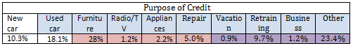
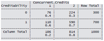
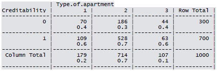
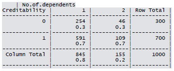
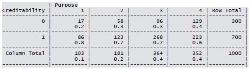
Proportions of applicants belonging to each classification of a categorical variable are shown in the following table (below). The pink shadings indicate that these levels have too few observations and the levels are merged for final analysis.
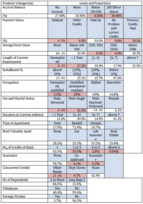
Since most of the predictors are categorical with several levels, the full cross-classification of all variables will lead to zero observations in many cells. Hence we need to reduce the table size. For details of variable names and classification see Appendix 1.
Depending on the cell proportions given in the one-way table above two or more cells are merged for several categorical predictors. We present below the final classification for the predictors that may potentially have any influence on Creditability
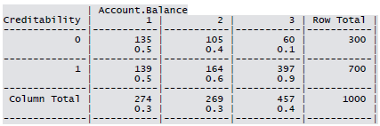
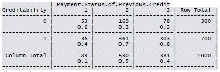
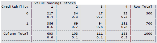
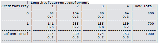
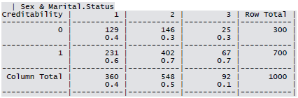
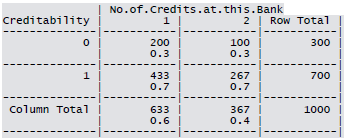
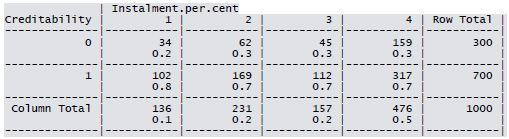
Cross-tabulation of the 9 predictors as defined above with Creditability is shown below. The proportions shown in the cells are column proportions and so are the marginal proportions. For example, 30% of 1000 applicants have no account and another 30% have no balance while 40% have some balance in their account. Among those who have no account 135 are found to be Creditable and 139 are found to be Non-Creditable. In the group with no balance in their account, 40% were found to be on-Creditable whereas in the group having some balance only 1% are found to be Non-Creditable.
Sample R code for creating K1 x K2 contingency table.

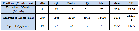
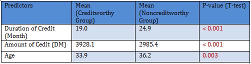
Summary for the continuous variables:
Sample R code for Descriptive Statistics.
Distribution of the continuous variables:
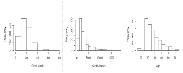
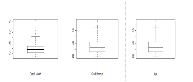
All the three variables show marked positive skewness. Boxplots bear this out even more clearly.
In preparation of predictors to use in building a logistic regression model, we consider bivariate association of the response (Creditability) with the categorical predictors.
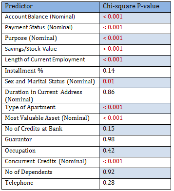
Since the number of predictors in this problem is not very high, it is possible to look into the dependency of the response (Creditability) on each of them individually. The following table summarizes the chi-square p-values for each contingency table. Note that among the sample of size 1000, 700 were Creditable and 300 Non-Creditable. This classification is based on the Bank’s opinion on the actual applicants.
Only significant predictors are to be included in the logistic regression model. Since there are 1000 observations 50:50 cross-validation scheme is tried:
Sample R code for
50:50 cross-validation data creation.
1000 observations are randomly partitioned into two equal sized subsets – Training and Test data. A logistic model is fit to the Training set.
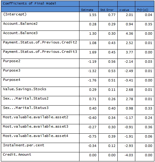
Results are given below, shaded rows indicate variables not significant at 10% level.
Sample R code for for
Logistic Model building with Training data
and assessing for Test data.
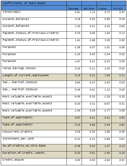
R output:
Null deviance: 598.536 on 499 degrees of freedom
Residual deviance: 464.01 on 477 degrees of freedom
AIC: 510.01
Removing the nonsignificant variables a second logistic regression is fit to the data.
R output:
Null deviance: 598.53 on 499 degrees of freedom
Residual deviance: 472.12 on 483 degrees of freedom
AIC: 506.12
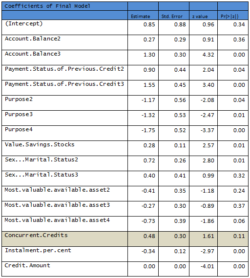
Need to remove another variable to come up with a model where all predictors are significant at 10% level.
R output:
Null deviance: 598.53 on 499 degrees of freedom
Residual deviance: 474.67 on 484 degrees of freedom
AIC: 506.67
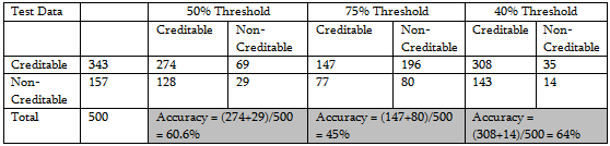
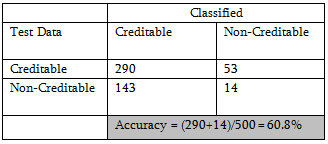
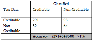
This model is recommended as the final model based on the Training Data. Final performance of a model is evaluated by considering the classification power. Following are a few tables defined at different thresholds of classification.
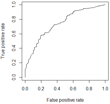
Following figure shows the performance of the classifier through ROC curve.
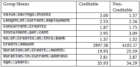
For discriminant analysis all the predictors are not used. Only the continuous variables and the ordinal variables are used as for the nominal variables there will be no concept of group means and linear discriminants will be difficult to interpret. The predictors are assumed to have a multivariate normal distribution.
Sample R code for
Discriminant Analysis.
Prior probability was taken as observed in the Training sample:
71.4% Creditable and 28.6% Non-creditable
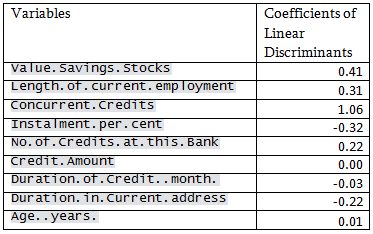
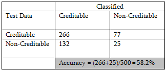
Neither logistic regression nor discriminant analysis is performing well for this data. The reason DA may not do well is that, most of the predictors are categorical and nominal predictors are not used in this analysis.
Sample R code for
Tree method.
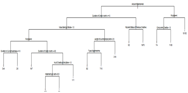
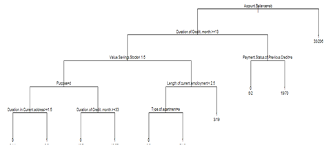
Both categorical and continuous predictors are used for binary classification. Using rpart{library=rpart}, the following tree is obtained without any pruning.
R output:
n= 500
node), split, n, loss, yval, (yprob)
* denotes terminal node
1) root 500 143 1 (0.28600000 0.71400000)
2) Account.Balance=1,2 261 110 1 (0.42145594 0.57854406)
4) Duration.of.Credit..month.>=13 165 79 0 (0.52121212 0.47878788)
8) Value.Savings.Stocks< 1.5 111 43 0 (0.61261261 0.38738739)
16) Purpose=4 45 9 0 (0.80000000 0.20000000)
32) Duration.in.Current.address>=1.5 38 4 0 (0.89473684 0.10526316) *
33) Duration.in.Current.address< 1.5 7 2 1 (0.28571429 0.71428571) *
17) Purpose=1,2,3 66 32 1 (0.48484848 0.51515152)
34) Duration.of.Credit..month.>=33 26 7 0 (0.73076923 0.26923077) *
35) Duration.of.Credit..month.< 33 40 13 1 (0.32500000 0.67500000)
70) No.of.Credits.at.this.Bank< 1.5 28 12 1 (0.42857143 0.57142857)
140) Instalment.per.cent>=2.5 17 7 0 (0.58823529 0.41176471) *
141) Instalment.per.cent< 2.5 11 2 1 (0.18181818 0.81818182) *
71) No.of.Credits.at.this.Bank>=1.5 12 1 1 (0.08333333 0.91666667) *
9) Value.Savings.Stocks>=1.5 54 18 1 (0.33333333 0.66666667)
18) Length.of.current.employment< 2.5 32 15 1 (0.46875000 0.53125000)
36) Type.of.apartment=1 10 2 0 (0.80000000 0.20000000) *
37) Type.of.apartment=2,3 22 7 1 (0.31818182 0.68181818) *
19) Length.of.current.employment>=2.5 22 3 1 (0.13636364 0.86363636) *
5) Duration.of.Credit..month.< 13 96 24 1 (0.25000000 0.75000000)
10) Payment.Status.of.Previous.Credit=1 7 2 0 (0.71428571 0.28571429) *
11) Payment.Status.of.Previous.Credit=2,3 89 19 1 (0.21348315 0.78651685) *
3) Account.Balance=3 239 33 1 (0.13807531 0.86192469)
6) Purpose=4 72 18 1 (0.25000000 0.75000000)
12) Concurrent.Credits< 1.5 11 4 0 (0.63636364 0.36363636) *
13) Concurrent.Credits>=1.5 61 11 1 (0.18032787 0.81967213) *
7) Purpose=1,2,3 167 15 1 (0.08982036 0.91017964) *
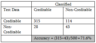
Applying the procedure on Test data, classification probability shows improvement.
The CP table is as follows:
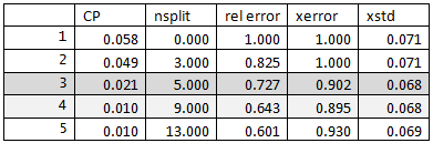
Following is the result for pruning the above tree for cross-validated classification error rate 90%.
n= 500
node), split, n, loss, yval, (yprob)
* denotes terminal node
1) root 500 143 1 (0.2860000 0.7140000)
2) Account.Balance=1,2 261 110 1 (0.4214559 0.5785441)
4) Duration.of.Credit..month.>=13 165 79 0 (0.5212121 0.4787879)
8) Value.Savings.Stocks< 1.5 111 43 0 (0.6126126 0.3873874)
16) Purpose=4 45 9 0 (0.8000000 0.2000000)
32) Duration.in.Current.address>=1.5 38 4 0 (0.8947368 0.1052632) *
33) Duration.in.Current.address< 1.5 7 2 1 (0.2857143 0.7142857) *
17) Purpose=1,2,3 66 32 1 (0.4848485 0.5151515)
34) Duration.of.Credit..month.>=33 26 7 0 (0.7307692 0.2692308) *
35) Duration.of.Credit..month.< 33 40 13 1 (0.3250000 0.6750000) *
9) Value.Savings.Stocks>=1.5 54 18 1 (0.3333333 0.6666667)
18) Length.of.current.employment< 2.5 32 15 1 (0.4687500 0.5312500)
36) Type.of.apartment=1 10 2 0 (0.8000000 0.2000000) *
37) Type.of.apartment=2,3 22 7 1 (0.3181818 0.6818182) *
19) Length.of.current.employment>=2.5 22 3 1 (0.1363636 0.8636364) *
5) Duration.of.Credit..month.< 13 96 24 1 (0.2500000 0.7500000)
10) Payment.Status.of.Previous.Credit=1 7 2 0 (0.7142857 0.2857143) *
11) Payment.Status.of.Previous.Credit=2,3 89 19 1 (0.2134831 0.7865169) *
3) Account.Balance=3 239 33 1 (0.1380753 0.8619247) *
There is minor improvement in accuracy % also
Conclusion: For this data set tree-based method seems to be working better than logistic regression or discriminant analysis.
Sample R code for
Random Forest.
Completely unsupervised random forest method on Training data with ntree = 200 leads to the following error plot:
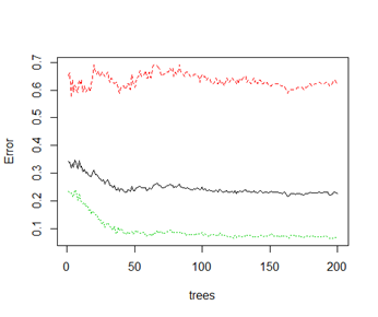
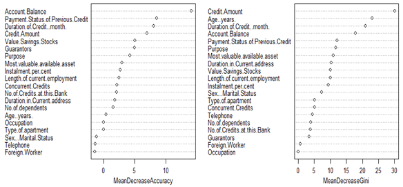
Importance of predictors are given in the following dotplot.
which gives rise to the following classification table:
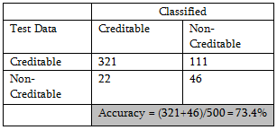
With judicious choice of more important predictors, further improvement in accuracy is possible. But as improvement is slight, no attempt is made for supervised random forest.
Ultimately these statistical decisions must be translated into profit consideration for the bank. Let us assume that a correct decision of the bank would result in 35% profit at the end of 5 years. A correct decision here means that the bank predicts an application to be good or credit-worthy and it actually turns out to be credit worthy. When the opposite is true, i.e. bank predicts the application to be good but it turns out to be bad credit, then the loss is 100%. If the bank predicts an application to be non-creditworthy, then loan facility is not extended to that applicant and bank does not incur any loss (opportunity loss is not considered here). The cost matrix, therefore, is as follows:
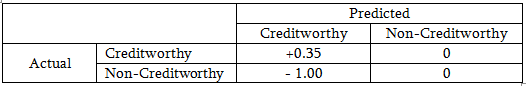
Out of 1000 applicants, 70% are creditworthy. A loan manager without any model would incur [0.7*0.35 + 0.3 (-1)] = - 0.055 or 0.055 unit loss. If the average loan amount is 3200 DM (approximately), then the total loss will be 1760000 DM and per applicant loss is 176 DM.
Logistic regression model performance:
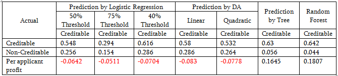
Tree-based classification and random forest show a per unit profit; other methods are not doing well.
|
Variable |
Description |
Categories |
Score |
rel. frequency |
|
|
good |
bad |
||||
|
kredit |
Creditability: |
||||
|
laufkont |
Balance of current account |
no balance or debit |
2 |
35.00 |
23.43 |
|
0 <= ... < 200 DM |
3 |
4.67 |
7.00 |
||
|
... >= 200 DM or checking account for at least 1 year |
4 |
15.33 |
49.71 |
||
|
no running account |
1 |
45.00 |
19.86 |
||
|
laufzeit |
Duration in months (metric) |
||||
|
dlaufzeit |
Duration in months (categorized) |
<=6 |
10 |
3.00 |
10.43 |
|
6 < ... <= 12 |
9 |
22.33 |
30.00 |
||
|
12 < ... <= 18 |
8 |
18.67 |
18.71 |
||
|
18 < ... <= 24 |
7 |
22.00 |
22.57 |
||
|
24 < ... <= 30 |
6 |
6.33 |
5.43 |
||
|
30 < ... <= 36 |
5 |
12.67 |
6.86 |
||
|
36 < ... <= 42 |
4 |
1.67 |
1.71 |
||
|
42 < ... <= 48 |
3 |
10.67 |
3.14 |
||
|
48 < ... <= 54 |
2 |
0.33 |
0.14 |
||
|
> 54 |
1 |
2.33 |
1.00 |
||
|
moral |
Payment of previous credits |
no previous credits / paid back all previous credits |
2 |
56.33 |
51.57 |
|
paid back previous credits at this bank |
4 |
16.67 |
34.71 |
||
|
no problems with current credits at this bank |
3 |
9.33 |
8.57 |
||
|
hesitant payment of previous credits |
0 |
8.33 |
2.14 |
||
|
problematic running account / there are further credits running but at other banks |
1 |
9.33 |
3.00 |
||
|
verw |
Purpose of credit |
new car |
1 |
5.67 |
12.29 |
|
used car |
2 |
19.33 |
17.57 |
||
|
items of furniture |
3 |
20.67 |
31.14 |
||
|
radio / television |
4 |
1.33 |
1.14 |
||
|
household appliances |
5 |
2.67 |
2.00 |
||
|
repair |
6 |
7.33 |
4.00 |
||
|
education |
7 |
0.00 |
0.00 |
||
|
vacation |
8 |
0.33 |
1.14 |
||
|
retraining |
9 |
11.33 |
9.00 |
||
|
business |
10 |
1.67 |
1.00 |
||
|
other |
0 |
29.67 |
20.71 |
||
|
Hoehe |
Amount of credit in "Deutsche Mark" (metric) |
||||
|
dhoehe |
Amount of credit in DM (categorized) |
<=500 |
10 |
1.00 |
2.14 |
|
500 < ... <= 1000 |
9 |
11.33 |
9.14 |
||
|
1000 < ... <= 1500 |
8 |
17.00 |
19.86 |
||
|
1500 < ... <= 2500 |
7 |
19.67 |
24.57 |
||
|
2500 < ... <= 5000 |
6 |
25.00 |
28.57 |
||
|
5000 < ... <= 7500 |
5 |
11.33 |
9.71 |
||
|
7500 < ... <= 10000 |
4 |
6.67 |
3.71 |
||
|
10000 < ... <= 15000 |
3 |
7.00 |
2.00 |
||
|
15000 < ... <= 20000 |
2 |
1.00 |
0.29 |
||
|
> 20000 |
1 |
0.00 |
0.00 |
||
|
sparkont |
Value of savings or stocks |
< 100,- DM |
2 |
11.33 |
9.86 |
|
100,- <= ... < 500,- DM |
3 |
3.67 |
7.43 |
||
|
500,- <= ... < 1000,- DM |
4 |
2.00 |
6.00 |
||
|
>= 1000,- DM |
5 |
10.67 |
21.57 |
||
|
not available / no savings |
1 |
72.33 |
55.14 |
||
|
beszeit |
Has been employed by current employer for |
unemployed |
1 |
7.67 |
5.57 |
|
<= 1 year |
2 |
23.33 |
14.57 |
||
|
1 <= ... < 4 years |
3 |
34.67 |
33.57 |
||
|
4 <= ... < 7 years |
4 |
13.00 |
19.29 |
||
|
>= 7 years |
5 |
21.33 |
27.00 |
||
|
rate |
Instalment in % of available income |
>= 35 |
1 |
11.33 |
14.57 |
|
25 <= ... < 35 |
2 |
20.67 |
24.14 |
||
|
20 <= ... < 25 |
3 |
15.00 |
16.00 |
||
|
< 20 |
4 |
53.00 |
45.29 |
||
|
famges |
Marital Status / Sex |
male: divorced / living apart |
1 |
6.67 |
4.29 |
|
male: single |
2 |
36.33 |
28.72 |
||
|
male: married / widowed |
3 |
48.67 |
57.43 |
||
|
female: |
4 |
8.33 |
9.57 |
||
|
buerge |
Further debtors / Guarantors |
none |
1 |
90.67 |
90.71 |
|
Co-Applicant |
2 |
6.00 |
3.29 |
||
|
Guarantor |
3 |
3.33 |
6.00 |
||
|
wohnzeit |
Living in current household for |
< 1 year |
1 |
12.00 |
13.43 |
|
1 <= ... < 4 years |
2 |
32.33 |
30.14 |
||
|
4 <= ... < 7 years |
3 |
14.33 |
15.14 |
||
|
>= 7 years |
4 |
41.33 |
41.29 |
||
|
verm |
Most valuable available assets |
Ownership of house or land |
4 |
22.33 |
12.43 |
|
Savings contract with a building society / Life insurance |
3 |
34.00 |
32.86 |
||
|
Car / Other |
2 |
23.67 |
23.00 |
||
|
not available / no assets |
1 |
20.00 |
31.71 |
||
|
alter |
Age in years (metric) |
||||
|
dalter |
Age in years (categorized) |
0 <= ... <= 25 |
1 |
26.67 |
15.71 |
|
26 <= ... <= 39 |
2 |
47.33 |
52.72 |
||
|
40 <= ... <= 59 |
3 |
21.67 |
26.14 |
||
|
60 <= ... <= 64 |
5 |
2.33 |
3.00 |
||
|
>= 65 |
4 |
2.00 |
2.43 |
||
|
weitkred |
Further running credits |
at other banks |
1 |
19.00 |
11.71 |
|
at department store or mail order house |
2 |
6.33 |
4.00 |
||
|
no further running credits |
3 |
74.67 |
84.29 |
||
|
wohn |
Type of apartment |
rented flat |
2 |
62.00 |
75.43 |
|
owner-occupied flat |
3 |
14.67 |
9.14 |
||
|
free apartment |
1 |
23.33 |
15.57 |
||
|
bishkred |
Number of previous credits at this bank (including the running one) |
one |
1 |
66.67 |
61.86 |
|
two or three |
2 |
30.67 |
34.43 |
||
|
four or five |
3 |
2.00 |
3.14 |
||
|
six or more |
4 |
0.67 |
0.57 |
||
|
beruf |
Occupation |
unemployed / unskilled with no permanent residence |
1 |
2.33 |
2.14 |
|
unskilled with permanent residence |
2 |
18.67 |
20.57 |
||
|
skilled worker / skilled employee / minor civil servant |
3 |
62.00 |
63.43 |
||
|
executive / self-employed / higher civil servant |
4 |
17.00 |
13.86 |
||
|
pers |
Number of persons entitled to maintenance |
0 to 2 |
2 |
84.67 |
84.43 |
|
3 and more |
1 |
15.33 |
15.57 |
||
|
telef |
Telephone |
no |
1 |
62.33 |
58.43 |
|
yes |
2 |
37.67 |
41.57 |
||
|
gastarb |
Foreign worker |
yes |
1 |
1.33 |
4.71 |
|
no |
2 |
98.67 |
95.29 |
||
Data and additional description may be found here:
https://www.stat.uni-muenchen.de/service/datenarchiv/kredit/kredit_e.html [4]
Links:
[1] https://onlinecourses.science.psu.edu/stat857/sites/onlinecourses.science.psu.edu.stat857/files/german_credit.csv
[2] https://onlinecourses.science.psu.edu/stat857/sites/onlinecourses.science.psu.edu.stat857/files/Training50.csv
[3] https://onlinecourses.science.psu.edu/stat857/sites/onlinecourses.science.psu.edu.stat857/files/Test50.csv
[4] https://www.stat.uni-muenchen.de/service/datenarchiv/kredit/kredit_e.html