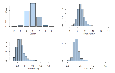
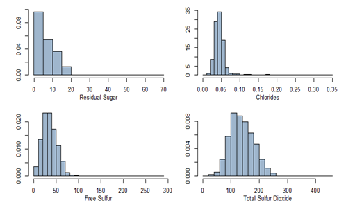
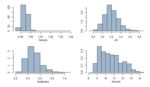
All variables are summarized and univariate analysis with plots are shown below.
Sample R code for EDA
attach(WhiteWine)
par(mfrow=c(2,2), oma = c(1,1,0,0) + 0.1, mar = c(3,3,1,1) + 0.1)
barplot((table(quality)), col=c("slateblue4", "slategray", "slategray1", "slategray2", "slategray3", "skyblue4"))mtext("Quality", side=1, outer=F, line=2, cex=0.8)truehist(fixed.acidity, h = 0.5, col="slategray3")
mtext("Fixed Acidity", side=1, outer=F, line=2, cex=0.8)truehist(volatile.acidity, h = 0.05, col="slategray3")
mtext("Volatile Acidity", side=1, outer=F, line=2, cex=0.8)truehist(citric.acid, h = 0.1, col="slategray3")
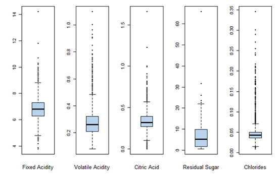
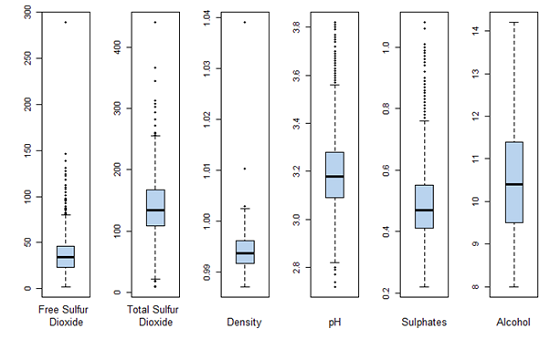
mtext("Citric Acid", side=1, outer=F, line=2, cex=0.8)par(mfrow=c(1,5), oma = c(1,1,0,0) + 0.1, mar = c(3,3,1,1) + 0.1)
boxplot(fixed.acidity, col="slategray2", pch=19)
mtext("Fixed Acidity", cex=0.8, side=1, line=2)boxplot(volatile.acidity, col="slategray2", pch=19)
mtext("Volatile Acidity", cex=0.8, side=1, line=2)boxplot(citric.acid, col="slategray2", pch=19)
mtext("Citric Acid", cex=0.8, side=1, line=2)boxplot(residual.sugar, col="slategray2", pch=19)
mtext("Residual Sugar", cex=0.8, side=1, line=2)boxplot(chlorides, col="slategray2", pch=19)
mtext("Chlorides", cex=0.8, side=1, line=2)
Boxplots for each of the variables as another indicator of spread.
Sample R code for Summary Statistics & Correlations
summary(WhiteWine)
library("psych", lib.loc="C:/Users/sbasu/Documents/R/R-3.1.0/library")describe(WhiteWine)
cor(WhiteWine[,-12])
cor(WhiteWine[,-12], method="spearman")
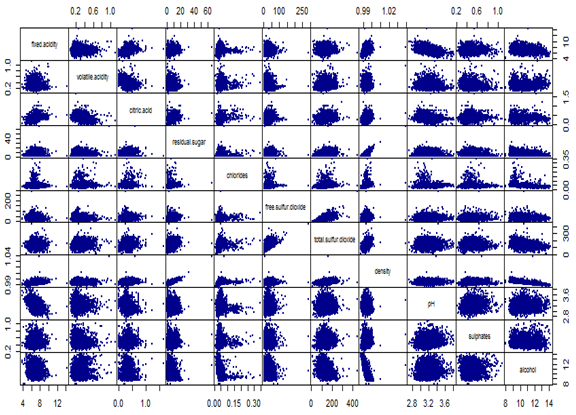
pairs(WhiteWine[,-12], gap=0, pch=19, cex=0.4, col="darkblue")
title(sub="Scatterplot of Chemical Attributes", cex=0.8)
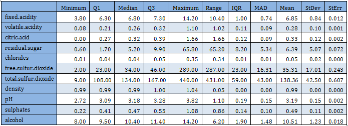
These observations are supported by the summary statistics also, as shown in the following table:
Range is much larger compared to the IQR. Mean is usually greater than the median. These observations indicate that there are outliers in the data set and before any analysis is performed outliers must be taken care of.
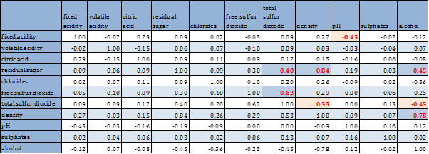
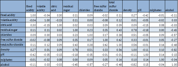
Next we look at the bivariate analysis, including all pairwise scatterplot and correlation coefficients. Since the variables have non-normal distribution, we have considered both person and spearman rank correlations.
Pearson’s correlation and rank correlations are very close, hence only the former is considered. High correlations (≥ 40% in absolute value) are identified and marked in red. Pairwise scatterplots are also shown below.
Sample R code for Preparing Data
limout <- rep(0,11)
for (i in 1:11){t1 <- quantile(WhiteWine[,i], 0.75)
t2 <- IQR(WhiteWine[,i], 0.75)
limout[i] <- t1 + 1.5*t2
}
WhiteWineIndex <- matrix(0, 4898, 11)
for (i in 1:4898)
for (j in 1:11){if (WhiteWine[i,j] > limout[j]) WhiteWineIndex[i,j] <- 1
}
WWInd <- apply(WhiteWineIndex, 1, sum)
WhiteWineTemp <- cbind(WWInd, WhiteWine)
Indexes <- rep(0, 208)
j <- 1
for (i in 1:4898){if (WWInd[i] > 0) {Indexes[j]<- ij <- j + 1}
else j <- j
}
WhiteWineLib <-WhiteWine[-Indexes,] # Inside of Q3+1.5IQR
indexes = sample(1:nrow(WhiteWineLib), size=0.5*nrow(WhiteWineLib))
WWTrain50 <- WhiteWineLib[indexes,]
WWTest50 <- WhiteWineLib[-indexes,]
Possibly the most important step in data preparation is to identify outliers. Since this is a multivariate data, we consider only those points which do not have any predictor variable value to be outside of limits constructed by boxplots. The following rule is applied:
The rationale behind this rule is that the extreme outliers are all on the higher end of the values and the distributions are all positively skewed. Application of this rule reduces the data size from 4899 to 4074.
Data is randomly divided into Training data and Test Data of equal sizes (50% each).