 In this example of data mining for knowledge discovery we consider a classification problem with a large number of objects to be classified based on many attributes. A set of 40 characters or attributes are measured on 5500 items which belong to 11 different categories of varied textures. Textures include a grass lawn, pressed calf leather, handmade paper, cotton canvas, etc. All of the attributes are measured on a continuous scale. Data are obtained from (https://sci2s.ugr.es/keel/dataset.php?cod=72#sub2 [1])
Pattern recognition and Classification of 5500 objects into 11 classes based on 40 attributes
Data Files for this case (right-click and "save as" ) :
Texture.csv [2] - full dataset
| TXTrain1.csv [3] TXTrain2.csv [4] TXTrain3.csv [5] TXTrain4.csv [6] TXTrain5.csv [7] TXTrain6.csv [8] TXTrain7.csv [9] TXTrain8.csv [10] TXTrain9.csv [11] TXTrain10.csv [12] |
TXTest1.csv [13] TXTest2.csv [14] TXTest3.csv [15] TXTest4.csv [16] TXTest5.csv [17] TXTest6.csv [18] TXTest7.csv [19] TXTest8.csv [20] TXTest9.csv [21] TXTest10.csv [22] |
Texture.zip [23] - all data files above together in a .zip file for convenience
Classification problem may be treated as a special type of regression problem where, based on the values of the predictors, each observation is placed into one and only one of the categories. Probability that the ith object will be placed into one of the j categories is 1, for all i = 1, … n. Each object has a different probability to be placed into different classes and is put into the class which maximizes this probability.
Performance of a classification rule is measured through the mis-classification probability. Following techniques of classification are applied here
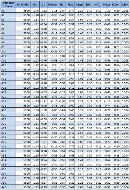
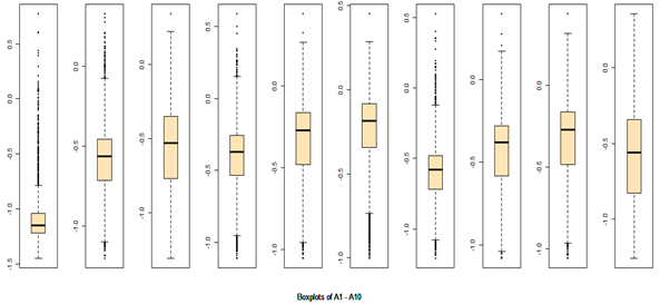
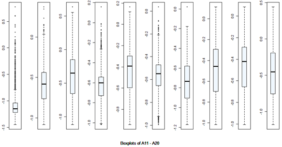
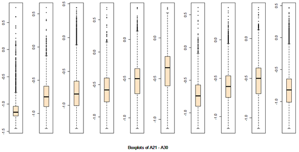
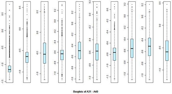
There are 40 predictors in the data. Univariate descriptive statistics and the box-plots are shown below.
R codes for
Data Preparation and
Exploratory Data Analysis
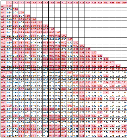
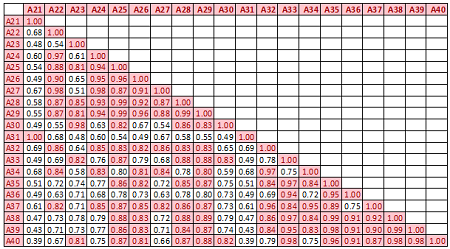
Descriptive statistics Boxplots From the above univariate exercises, it is clear that several of the 40 attributes have outliers of varied proportion. In order to include as many rows as possible, but eliminating the extreme outliers, all data points (rows) were included, which do not contain any outlier value in any of the 40 predictors, outliers being defined as a value outside of [Q1-3IQR, Q3+3IQR] limits. This eliminates 128 rows. A more conservative approach is where the outlier is defined to be a point outside of the limit [Q1-1.5IQR, Q3+1.5IQR]. In this case, 1060 rows would have been removed. While looking at the correlation matrix it was found that there is a very high degree of dependency among the predictor variables. The red highlighted cells all show very high degree of dependency and it is all in the positive direction.
R codes for
Principal Component Analysis
With such a high degree of dependency it is recommended that a PCA is done on the data and only the top few components are used for classification.
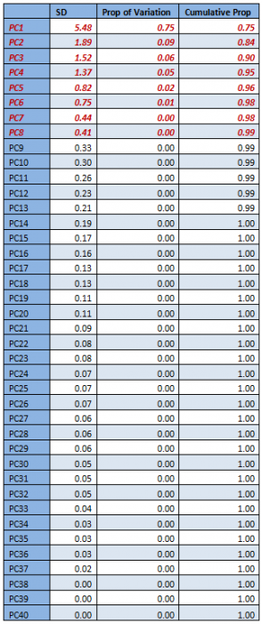
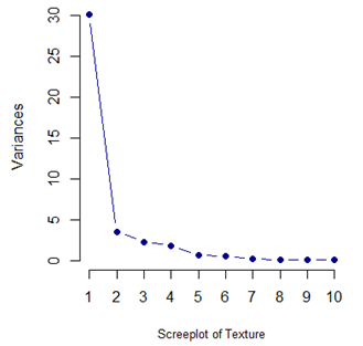
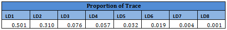
From the table and the screeplot above it is clear that it is sufficient to consider only the first 8 PCs. They are given below.
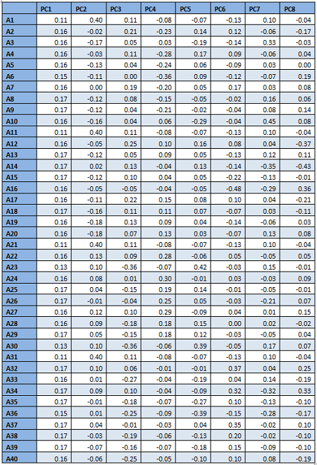
For classification, therefore, only the first 8 PCs will be used, instead of all the 40 attributes.
Since data set is large enough, 10-fold cross-validation is applied to evaluate model performance. After removing the outliers 5372 observations are included in the master data and the first 8 principal components are used for prediction. For each observation (row) a score corresponding to each PC is computed and this is the value of the predictors (PCs) used to evaluate model performance. Hence the master data used has 5372 rows (observations) and 8 predictors and one response (total of 9 columns) indicating the classes each observation belongs to.
Data is divided into 10 sets randomly of which 9 sets have 537 observations and the last set has 539 observations. Training data is formed by taking 9 sets at a time and leave one set out as the Test data. Hence 10 different combinations of Training and Test sets are formed. On each of Training and Test pair a technique is applied and evaluated. Final evaluation of the technique is determined by the average mis-classification probability over the 10 Test sets.
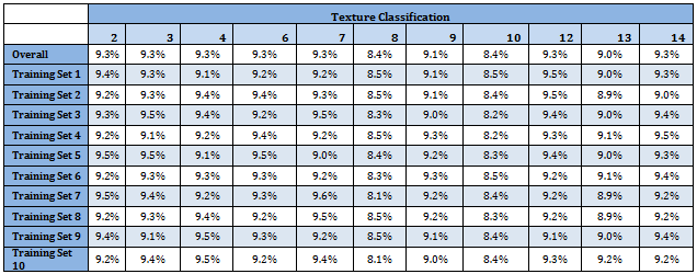
Following table shows classification proportion in the Master data as well as in the Training data sets. Distribution of different classes is almost identical over the data sets. Moreover all categories have almost uniform representation
R codes for
Discriminant Analysis
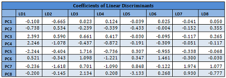
Since PCs are linear combinations of original variables, they may also be assumed to follow multivariate normal distribution. For each Training set a linear discriminant function is developed using all 8 PCs. Prior probability distribution for each Training set is very similar as given in the table above.
Details are given for the Training Data 1:
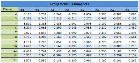
Results from other Training sets are also very similar and are not shown here. In the following table misclassification probabilities in Training and Test sets created for the 10-fold cross-validation are shown.
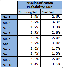
Therefore overall misclassification probability of the 10-fold cross-validation is 2.55%, which is the mean misclassification probability of the Test sets.
Note that for Sets 5, 7, 8 and 9 mis-classification probability in Test set is less than that in the corresponding Training set. This may seem fallacious; however, several points to be noted here. Training set size is much larger compared to Test set. With 11 classes in Test sets, each class has sometimes even fewer than 40 representations. This might lead to the standard error of probability of misclassification to be relatively higher, in turn leading to apparent counter-intuitive results. Average error of Training set is 2.54%.
Overall results indicate accurate and stable classification rules.
For this method k = 7 is used, i.e. 7 nearest neighbours are used to predict class membership of each observation in the Test set. Following is the misclassification error rate for Test sets.
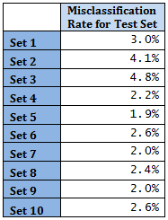
Overall error rate is 3.0%. This value is comparable to the LDA error rate.
R codes for
Tree Based Algorithms
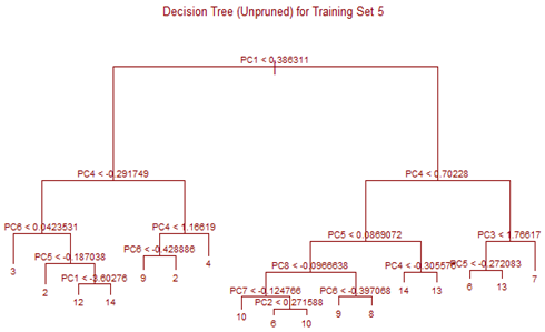
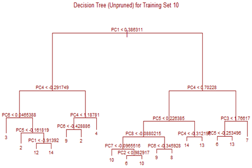
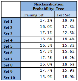
Unsupervised tree algorithm is applied to all Training sets and misclassification probability was calculated for both the Training and Test sets. All the Training Sets give rise to very similar decision trees. Three representative trees are shown below as examples. Following table summarizes the misclassification probabilities for Tree classification Therefore overall mis-classification probability of the 10-fold cross-validation is 17.9%, which is the mean mis-classification probability of the Test sets. Pruning was tried for this decision tree, but it did not improve the result. At the first glance this high error rate compared to k-NN and LDA looks surprising. LDA uses only linear classifier all over the sample space, but Tree procedure recursively partitions the sample space to reduce mis-classification error. It is therefore expected that Tree procedure will always give better results than LDA. However, it is to be noted that LDA takes into account linear combinations of the predictors, whereas Tree always divides the sample space into splits parallel to the axes. If separation is along any other line, Tree wil not be able to capture that. This is exactly what is happening here.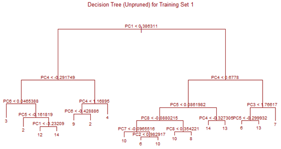
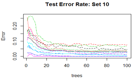
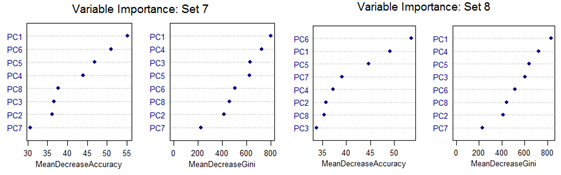
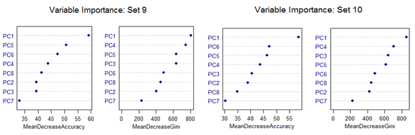
High mis-classification error rate is corrected to a large extent by using Random Forest. Unsupervised random forest method is applied to each Training set and both Out-of-Bag error rate and Test error rate are calculated for error or mis-classification corresponding to each of the 11 categories. Variable importance plots are also shown. All results are for ntree = 100. Number of variables tried at each split is 2.
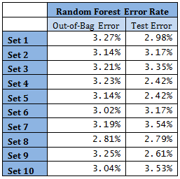
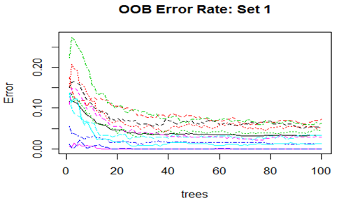
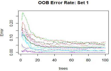
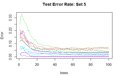
Convergence of the errors are shown for two Sets only since behaviour of the error is very similar for all the 10 Sets random forest technique was applied. For Set 1 both the Out-of-Bag error rate and Test error rate are shown.
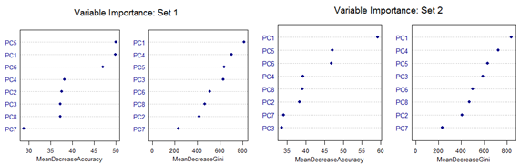
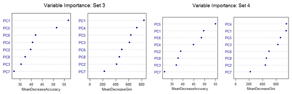
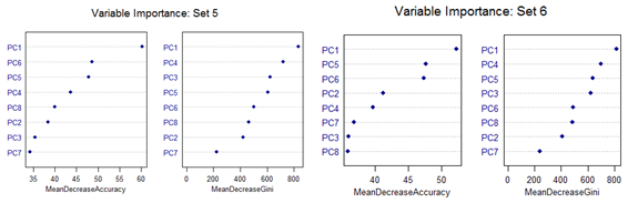
However, there are slight differences in the variable importance plots. All the plots are shown below. It is clear from the plots below that PC1, PC5 and PC6 are the primary influential variables, but they appear in different order in different cross-validation sets.
All the 11 different categories can be separated by various classification methods with almost similar misclassification error rates. Classification Tree-based method shows less than optimal performance. But this can be improved by application of Random Forest or Oblique Tree method.
Links:
[1] https://sci2s.ugr.es/keel/dataset.php?cod=72#sub2
[2] https://onlinecourses.science.psu.edu/stat857/sites/onlinecourses.science.psu.edu.stat857/files/Texture.csv
[3] https://onlinecourses.science.psu.edu/stat857/sites/onlinecourses.science.psu.edu.stat857/files/TXTrain1.csv
[4] https://onlinecourses.science.psu.edu/stat857/sites/onlinecourses.science.psu.edu.stat857/files/TXTrain2.csv
[5] https://onlinecourses.science.psu.edu/stat857/sites/onlinecourses.science.psu.edu.stat857/files/TXTrain3.csv
[6] https://onlinecourses.science.psu.edu/stat857/sites/onlinecourses.science.psu.edu.stat857/files/TXTrain4.csv
[7] https://onlinecourses.science.psu.edu/stat857/sites/onlinecourses.science.psu.edu.stat857/files/TXTrain5.csv
[8] https://onlinecourses.science.psu.edu/stat857/sites/onlinecourses.science.psu.edu.stat857/files/TXTrain6.csv
[9] https://onlinecourses.science.psu.edu/stat857/sites/onlinecourses.science.psu.edu.stat857/files/TXTrain7.csv
[10] https://onlinecourses.science.psu.edu/stat857/sites/onlinecourses.science.psu.edu.stat857/files/TXTrain8.csv
[11] https://onlinecourses.science.psu.edu/stat857/sites/onlinecourses.science.psu.edu.stat857/files/TXTrain9.csv
[12] https://onlinecourses.science.psu.edu/stat857/sites/onlinecourses.science.psu.edu.stat857/files/TXTrain10.csv
[13] https://onlinecourses.science.psu.edu/stat857/sites/onlinecourses.science.psu.edu.stat857/files/TXTest1.csv
[14] https://onlinecourses.science.psu.edu/stat857/sites/onlinecourses.science.psu.edu.stat857/files/TXTest2.csv
[15] https://onlinecourses.science.psu.edu/stat857/sites/onlinecourses.science.psu.edu.stat857/files/TXTest3.csv
[16] https://onlinecourses.science.psu.edu/stat857/sites/onlinecourses.science.psu.edu.stat857/files/TXTest4.csv
[17] https://onlinecourses.science.psu.edu/stat857/sites/onlinecourses.science.psu.edu.stat857/files/TXTest5.csv
[18] https://onlinecourses.science.psu.edu/stat857/sites/onlinecourses.science.psu.edu.stat857/files/TXTest6.csv
[19] https://onlinecourses.science.psu.edu/stat857/sites/onlinecourses.science.psu.edu.stat857/files/TXTest7.csv
[20] https://onlinecourses.science.psu.edu/stat857/sites/onlinecourses.science.psu.edu.stat857/files/TXTest8.csv
[21] https://onlinecourses.science.psu.edu/stat857/sites/onlinecourses.science.psu.edu.stat857/files/TXTest9.csv
[22] https://onlinecourses.science.psu.edu/stat857/sites/onlinecourses.science.psu.edu.stat857/files/TXTest10.csv
[23] https://onlinecourses.science.psu.edu/stat857/sites/onlinecourses.science.psu.edu.stat857/files/Texture.zip