Basic Statistical Concepts
Basic Statistical ConceptsThe Prerequisites Checklist page on the Department of Statistics website lists a number of courses that require a foundation of basic statistical concepts as a prerequisite. All of the graduate courses in the Master of Applied Statistics program heavily rely on these concepts and procedures. Therefore, it is imperative — after you study and work through this lesson — that you thoroughly understand all the material presented here. Students that do not possess a firm understanding of these basic concepts will struggle to participate successfully in any of the graduate-level courses above STAT 500. Courses such as STAT 501 - Regression Methods or STAT 502 - Analysis of Variance and Design of Experiments require and build from this foundation.
Review Materials
These review materials are intended to provide a review of key statistical concepts and procedures. Specifically, the lesson reviews:
- populations and parameters and how they differ from samples and statistics,
- confidence intervals and their interpretation,
- hypothesis testing procedures, including the critical value approach and the P-value approach,
- chi-square analysis,
- tests of proportion, and
- power analysis.
For instance, with regards to hypothesis testing, some of you may have learned only one approach — some the P-value approach, and some the critical value approach. It is important that you understand both approaches. If the P-value approach is new to you, you might have to spend a little more time on this lesson than if not.
Learning Objectives & Outcomes
Upon completion of this review of basic statistical concepts, you should be able to do the following:
-
Distinguish between a population and a sample.
-
Distinguish between a parameter and a statistic.
-
Understand the basic concept and the interpretation of a confidence interval.
-
Know the general form of most confidence intervals.
-
Be able to calculate a confidence interval for a population mean µ.
-
Understand how different factors affect the length of the t-interval for the population mean µ.
-
Understand the general idea of hypothesis testing -- especially how the basic procedure is similar to that followed for criminal trials conducted in the United States.
-
Be able to distinguish between the two types of errors that can occur whenever a hypothesis test is conducted.
-
Understand the basic procedures for the critical value approach to hypothesis testing. Specifically, be able to conduct a hypothesis test for the population mean µ using the critical value approach.
-
Understand the basic procedures for the P-value approach to hypothesis testing. Specifically, be able to conduct a hypothesis test for the population mean µ using the P-value approach.
- Understand the basic procedures for testing the independence of two categorical variables using a Chi-square test of independence.
- Be able to determine if a test contains enough power to make a reasonable conclusion using power analysis.
- Be able to use power analysis to calculate the number of samples required to achieve a specified level of power.
- Understand how a test of proportion can be used to assess whether a sample from a population represents the true proportion of the entire population.
Self-Assessment Procedure
- Review the concepts and methods on the pages in this section of this website.
- Download and complete the Self-Assessment Exam at the end of this section.
- Review the Self-Assessment Exam Solutions and determine your score.
A score below 70% suggests that the concepts and procedures that are covered in STAT 500 have not been mastered adequately. Students are strongly encouraged to take STAT 500, thoroughly review the materials that are covered in the sections above or take additional coursework that focuses on these foundations.
If you have struggled with the concepts and methods that are presented here, you will indeed struggle in any of the graduate-level courses included in the Master of Applied Statistics program above STAT 500 that expect and build on this foundation.
S.1 Basic Terminology
S.1 Basic TerminologyPopulation and Parameters
- Population
- A population is any large collection of objects or individuals, such as Americans, students, or trees about which information is desired.
- Parameter
- A parameter is any summary number, like an average or percentage, that describes the entire population.
The population mean \(\mu\) (the greek letter "mu") and the population proportion p are two different population parameters. For example:
- We might be interested in learning about \(\mu\), the average weight of all middle-aged female Americans. The population consists of all middle-aged female Americans, and the parameter is µ.
- Or, we might be interested in learning about p, the proportion of likely American voters approving of the president's job performance. The population comprises all likely American voters, and the parameter is p.
The problem is that 99.999999999999... % of the time, we don't — or can't — know the real value of a population parameter. The best we can do is estimate the parameter! This is where samples and statistics come in to play.
Samples and statistics
- Sample
- A sample is a representative group drawn from the population.
- Statistic
- A statistic is any summary number, like an average or percentage, that describes the sample.
The sample mean, \(\bar{x}\), and the sample proportion \(\hat{p}\) are two different sample statistics. For example:
- We might use \(\bar{x}\), the average weight of a random sample of 100 middle-aged female Americans, to estimate µ, the average weight of all middle-aged female Americans.
- Or, we might use \(\hat{p}\), the proportion in a random sample of 1000 likely American voters who approve of the president's job performance, to estimate p, the proportion of all likely American voters who approve of the president's job performance.
Because samples are manageable in size, we can determine the actual value of any statistic. We use the known value of the sample statistic to learn about the unknown value of the population parameter.
Example S.1.1
What was the prevalence of smoking at Penn State University before the 'no smoking' policy?
The main campus at Penn State University has a population of approximately 42,000 students. A research question is "What proportion of these students smoke regularly?" A survey was administered to a sample of 987 Penn State students. Forty-three percent (43%) of the sampled students reported that they smoked regularly. How confident can we be that 43% is close to the actual proportion of all Penn State students who smoke?
- The population is all 42,000 students at Penn State University.
- The parameter of interest is p, the proportion of students at Penn State University who smoke regularly.
- The sample is a random selection of 987 students at Penn State University.
- The statistic is the proportion, \(\hat{p}\), of the sample of 987 students who smoke regularly. The value of the sample proportion is 0.43.
Example S.1.2
Are the grades of college students inflated?
Let's suppose that there exists a population of 7 million college students in the United States today. (The actual number depends on how you define "college student.") And, let's assume that the average GPA of all of these college students is 2.7 (on a 4-point scale). If we take a random sample of 100 college students, how likely is it that the sampled 100 students would have an average GPA as large as 2.9 if the population average was 2.7?
- The population is equal to all 7 million college students in the United States today.
- The parameter of interest is µ, the average GPA of all college students in the United States today.
- The sample is a random selection of 100 college students in the United States.
- The statistic is the mean grade point average, \(\bar{x}\), of the sample of 100 college students. The value of the sample mean is 2.9.
Example S.1.3
Is there a linear relationship between birth weight and length of gestation?
Consider the relationship between the birth weight of a baby and the length of its gestation:
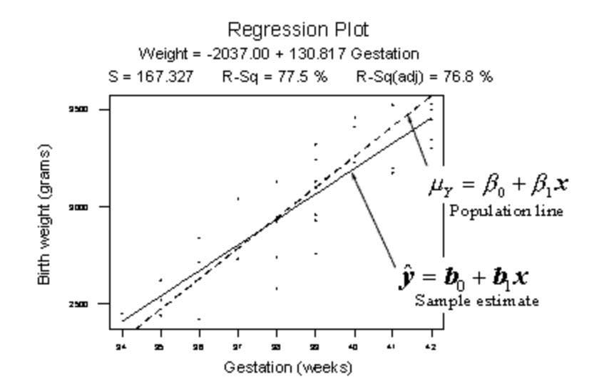
The dashed line summarizes the (unknown) relationship —\(\mu_Y = \beta_0+\beta_1x\)— between birth weight and gestation length of all births in the population. The solid line summarizes the relationship —\(\hat{y} = \beta_0+\beta_1x\)— between birth weight and gestation length in our random sample of 32 births. The goal of linear regression analysis is to use the solid line (the sample) in hopes of learning about the dashed line (the population).
Next... Confidence intervals and hypothesis tests
There are two ways to learn about a population parameter.
1) We can use confidence intervals to estimate parameters.
"We can be 95% confident that the proportion of Penn State students who have a tattoo is between 5.1% and 15.3%."
2) We can use hypothesis tests to test and ultimately draw conclusions about the value of a parameter.
"There is enough statistical evidence to conclude that the mean normal body temperature of adults is lower than 98.6 degrees F."
We review these two methods in the next two sections.
S.2 Confidence Intervals
S.2 Confidence IntervalsLet's review the basic concept of a confidence interval.
Suppose we want to estimate an actual population mean \(\mu\). As you know, we can only obtain \(\bar{x}\), the mean of a sample randomly selected from the population of interest. We can use \(\bar{x}\) to find a range of values:
\[\text{Lower value} < \text{population mean}\;\; \mu < \text{Upper value}\]
that we can be really confident contains the population mean \(\mu\). The range of values is called a "confidence interval."
Example S.2.1
Should using a hand-held cell phone while driving be illegal?
There is little doubt that you have seen numerous confidence intervals for population proportions reported in newspapers over the years.
For example, a newspaper report (ABC News poll, May 16-20, 2001) was concerned about whether or not U.S. adults thought using a hand-held cell phone while driving should be illegal. Of the 1,027 U.S. adults randomly selected for participation in the poll, 69% believed it should be illegal. The reporter claimed that the poll's "margin of error" was 3%. Therefore, the confidence interval for the (unknown) population proportion p is 69% ± 3%. That is, we can be really confident that between 66% and 72% of all U.S. adults think using a hand-held cell phone while driving a car should be illegal.
General Form of (Most) Confidence Intervals
The previous example illustrates the general form of most confidence intervals, namely:
$\text{Sample estimate} \pm \text{margin of error}$
The lower limit is obtained by:
$\text{the lower limit L of the interval} = \text{estimate} - \text{margin of error}$
The upper limit is obtained by:
$\text{the upper limit U of the interval} = \text{estimate} + \text{margin of error}$
Once we've obtained the interval, we can claim that we are really confident that the value of the population parameter is somewhere between the value of L and the value of U.
So far, we've been very general in our discussion of the calculation and interpretation of confidence intervals. To be more specific about their use, let's consider a specific interval, namely the "t-interval for a population mean µ."
(1-α)100% t-interval for the population mean \(\mu\)
If we are interested in estimating a population mean \(\mu\), it is very likely that we would use the t-interval for a population mean \(\mu\).
- t-Interval for a Population Mean
- The formula for the confidence interval in words is:
$\text{Sample mean} \pm (\text{t-multiplier} \times \text{standard error})$
- and you might recall that the formula for the confidence interval in notation is:
- $\bar{x}\pm t_{\alpha/2, n-1}\left(\dfrac{s}{\sqrt{n}}\right)$
Note that:
- the "t-multiplier," which we denote as \(t_{\alpha/2, n-1}\), depends on the sample size through n - 1 (called the "degrees of freedom") and the confidence level \((1-\alpha)\times100%\) through \(\frac{\alpha}{2}\).
- the "standard error," which is \(\frac{s}{\sqrt{n}}\), quantifies how much the sample means \(\bar{x}\) vary from sample to sample. That is, the standard error is just another name for the estimated standard deviation of all the possible sample means.
- the quantity to the right of the ± sign, i.e., "t-multiplier × standard error," is just a more specific form of the margin of error. That is, the margin of error in estimating a population mean µ is calculated by multiplying the t-multiplier by the standard error of the sample mean.
- the formula is only appropriate if a certain assumption is met, namely that the data are normally distributed.
Clearly, the sample mean \(\bar{x}\), the sample standard deviation s, and the sample size n are all readily obtained from the sample data. Now, we need to review how to obtain the value of the t-multiplier, and we'll be all set.
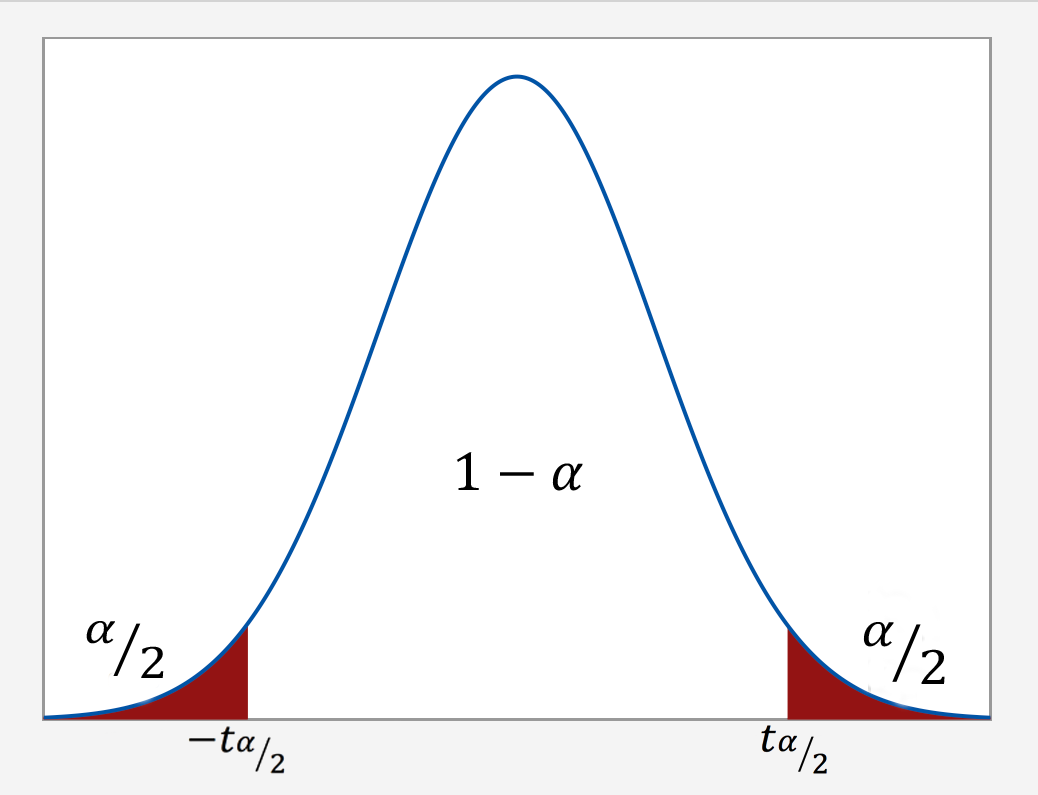
How is the t-multiplier determined?
As the following graph illustrates, we put the confidence level $1-\alpha$ in the center of the t-distribution. Then, since the entire probability represented by the curve must equal 1, a probability of α must be shared equally among the two "tails" of the distribution. That is, the probability of the left tail is $\frac{\alpha}{2}$ and the probability of the right tail is $\frac{\alpha}{2}$. If we add up the probabilities of the various parts $(\frac{\alpha}{2} + 1-\alpha + \frac{\alpha}{2})$, we get 1. The t-multiplier, denoted \(t_{\alpha/2}\), is the t-value such that the probability "to the right of it" is $\frac{\alpha}{2}$:
It should be no surprise that we want to be as confident as possible when we estimate a population parameter. This is why confidence levels are typically very high. The most common confidence levels are 90%, 95%, and 99%. The following table contains a summary of the values of \(\frac{\alpha}{2}\) corresponding to these common confidence levels. (Note that the"confidence coefficient" is merely the confidence level reported as a proportion rather than as a percentage.)
| Confidence Coefficient $(1-\alpha)$ | Confidence Level $(1-\alpha) \times 100$ | $(1-\dfrac{\alpha}{2})$ | $\dfrac{\alpha}{2}$ |
|---|---|---|---|
| 0.90 | 90% | 0.95 | 0.05 |
| 0.95 | 95% | 0.975 | 0.025 |
| 0.99 | 99% | 0.995 | 0.005 |
Minitab® – Using Software
The good news is that statistical software, such as Minitab, will calculate most confidence intervals for us.
Let's take an example of researchers who are interested in the average heart rate of male college students. Assume a random sample of 130 male college students were taken for the study.
The following is the Minitab Output of a one-sample t-interval output using this data.
One-Sample T: Heart Rate
Descriptive Statistics
| N | Mean | StDev | SE Mean | 95% CI for $\mu$ |
|---|---|---|---|---|
| 130 | 73.762 | 7.062 | 0.619 | (72.536, 74.987) |
$\mu$: mean of HR
In this example, the researchers were interested in estimating \(\mu\), the heart rate. The output indicates that the mean for the sample of n = 130 male students equals 73.762. The sample standard deviation (StDev) is 7.062 and the estimated standard error of the mean (SE Mean) is 0.619. The 95% confidence interval for the population mean $\mu$ is (72.536, 74.987). We can be 95% confident that the mean heart rate of all male college students is between 72.536 and 74.987 beats per minute.
Factors Affecting the Width of the t-interval for the Mean $\mu$
Think about the width of the interval in the previous example. In general, do you think we desire narrow confidence intervals or wide confidence intervals? If you are not sure, consider the following two intervals:
- We are 95% confident that the average GPA of all college students is between 1.0 and 4.0.
- We are 95% confident that the average GPA of all college students is between 2.7 and 2.9.
Which of these two intervals is more informative? Of course, the narrower one gives us a better idea of the magnitude of the true unknown average GPA. In general, the narrower the confidence interval, the more information we have about the value of the population parameter. Therefore, we want all of our confidence intervals to be as narrow as possible. So, let's investigate what factors affect the width of the t-interval for the mean \(\mu\).
Of course, to find the width of the confidence interval, we just take the difference in the two limits:
Width = Upper Limit - Lower Limit
What factors affect the width of the confidence interval? We can examine this question by using the formula for the confidence interval and seeing what would happen should one of the elements of the formula be allowed to vary.
\[\bar{x}\pm t_{\alpha/2, n-1}\left(\dfrac{s}{\sqrt{n}}\right)\]
What is the width of the t-interval for the mean? If you subtract the lower limit from the upper limit, you get:
\[\text{Width }=2 \times t_{\alpha/2, n-1}\left(\dfrac{s}{\sqrt{n}}\right)\]
Now, let's investigate the factors that affect the length of this interval. Convince yourself that each of the following statements is accurate:
- As the sample mean increases, the length stays the same. That is, the sample mean plays no role in the width of the interval.
- As the sample standard deviation s decreases, the width of the interval decreases. Since s is an estimate of how much the data vary naturally, we have little control over s other than making sure that we make our measurements as carefully as possible.
- As we decrease the confidence level, the t-multiplier decreases, and hence the width of the interval decreases. In practice, we wouldn't want to set the confidence level below 90%.
- As we increase the sample size, the width of the interval decreases. This is the factor that we have the most flexibility in changing, the only limitation being our time and financial constraints.
In Closing
In our review of confidence intervals, we have focused on just one confidence interval. The important thing to recognize is that the topics discussed here — the general form of intervals, determination of t-multipliers, and factors affecting the width of an interval — generally extend to all of the confidence intervals we will encounter in this course.
S.3 Hypothesis Testing
S.3 Hypothesis TestingIn reviewing hypothesis tests, we start first with the general idea. Then, we keep returning to the basic procedures of hypothesis testing, each time adding a little more detail.
The general idea of hypothesis testing involves:
- Making an initial assumption.
- Collecting evidence (data).
- Based on the available evidence (data), deciding whether to reject or not reject the initial assumption.
Every hypothesis test — regardless of the population parameter involved — requires the above three steps.
Example S.3.1
Is Normal Body Temperature Really 98.6 Degrees F?
Consider the population of many, many adults. A researcher hypothesized that the average adult body temperature is lower than the often-advertised 98.6 degrees F. That is, the researcher wants an answer to the question: "Is the average adult body temperature 98.6 degrees? Or is it lower?" To answer his research question, the researcher starts by assuming that the average adult body temperature was 98.6 degrees F.
Then, the researcher went out and tried to find evidence that refutes his initial assumption. In doing so, he selects a random sample of 130 adults. The average body temperature of the 130 sampled adults is 98.25 degrees.
Then, the researcher uses the data he collected to make a decision about his initial assumption. It is either likely or unlikely that the researcher would collect the evidence he did given his initial assumption that the average adult body temperature is 98.6 degrees:
- If it is likely, then the researcher does not reject his initial assumption that the average adult body temperature is 98.6 degrees. There is not enough evidence to do otherwise.
- If it is unlikely, then:
- either the researcher's initial assumption is correct and he experienced a very unusual event;
- or the researcher's initial assumption is incorrect.
In statistics, we generally don't make claims that require us to believe that a very unusual event happened. That is, in the practice of statistics, if the evidence (data) we collected is unlikely in light of the initial assumption, then we reject our initial assumption.
Example S.3.2
Criminal Trial Analogy
One place where you can consistently see the general idea of hypothesis testing in action is in criminal trials held in the United States. Our criminal justice system assumes "the defendant is innocent until proven guilty." That is, our initial assumption is that the defendant is innocent.
In the practice of statistics, we make our initial assumption when we state our two competing hypotheses -- the null hypothesis (H0) and the alternative hypothesis (HA). Here, our hypotheses are:
- H0: Defendant is not guilty (innocent)
- HA: Defendant is guilty
In statistics, we always assume the null hypothesis is true. That is, the null hypothesis is always our initial assumption.
The prosecution team then collects evidence — such as finger prints, blood spots, hair samples, carpet fibers, shoe prints, ransom notes, and handwriting samples — with the hopes of finding "sufficient evidence" to make the assumption of innocence refutable.
In statistics, the data are the evidence.
The jury then makes a decision based on the available evidence:
- If the jury finds sufficient evidence — beyond a reasonable doubt — to make the assumption of innocence refutable, the jury rejects the null hypothesis and deems the defendant guilty. We behave as if the defendant is guilty.
- If there is insufficient evidence, then the jury does not reject the null hypothesis. We behave as if the defendant is innocent.
In statistics, we always make one of two decisions. We either "reject the null hypothesis" or we "fail to reject the null hypothesis."
Errors in Hypothesis Testing
Did you notice the use of the phrase "behave as if" in the previous discussion? We "behave as if" the defendant is guilty; we do not "prove" that the defendant is guilty. And, we "behave as if" the defendant is innocent; we do not "prove" that the defendant is innocent.
This is a very important distinction! We make our decision based on evidence not on 100% guaranteed proof. Again:
- If we reject the null hypothesis, we do not prove that the alternative hypothesis is true.
- If we do not reject the null hypothesis, we do not prove that the null hypothesis is true.
We merely state that there is enough evidence to behave one way or the other. This is always true in statistics! Because of this, whatever the decision, there is always a chance that we made an error.
Let's review the two types of errors that can be made in criminal trials:
| Jury Decision | Truth | ||
|---|---|---|---|
| Not Guilty | Guilty | ||
| Not Guilty | OK | ERROR | |
| Guilty | ERROR | OK | |
Table S.3.2 shows how this corresponds to the two types of errors in hypothesis testing.
| Decision | Truth | ||
|---|---|---|---|
| Null Hypothesis | Alternative Hypothesis | ||
| Do not Reject Null | OK | Type II Error | |
| Reject Null | Type I Error | OK | |
Note that, in statistics, we call the two types of errors by two different names -- one is called a "Type I error," and the other is called a "Type II error." Here are the formal definitions of the two types of errors:
- Type I Error
- The null hypothesis is rejected when it is true.
- Type II Error
- The null hypothesis is not rejected when it is false.
There is always a chance of making one of these errors. But, a good scientific study will minimize the chance of doing so!
Making the Decision
Recall that it is either likely or unlikely that we would observe the evidence we did given our initial assumption. If it is likely, we do not reject the null hypothesis. If it is unlikely, then we reject the null hypothesis in favor of the alternative hypothesis. Effectively, then, making the decision reduces to determining "likely" or "unlikely."
In statistics, there are two ways to determine whether the evidence is likely or unlikely given the initial assumption:
- We could take the "critical value approach" (favored in many of the older textbooks).
- Or, we could take the "P-value approach" (what is used most often in research, journal articles, and statistical software).
In the next two sections, we review the procedures behind each of these two approaches. To make our review concrete, let's imagine that μ is the average grade point average of all American students who major in mathematics. We first review the critical value approach for conducting each of the following three hypothesis tests about the population mean $\mu$:
|
Type
|
Null
|
Alternative
|
|---|---|---|
|
Right-tailed
|
H0 : μ = 3
|
HA : μ > 3
|
|
Left-tailed
|
H0 : μ = 3
|
HA : μ < 3
|
|
Two-tailed
|
H0 : μ = 3
|
HA : μ ≠ 3
|
In Practice
-
We would want to conduct the first hypothesis test if we were interested in concluding that the average grade point average of the group is more than 3.
-
We would want to conduct the second hypothesis test if we were interested in concluding that the average grade point average of the group is less than 3.
-
And, we would want to conduct the third hypothesis test if we were only interested in concluding that the average grade point average of the group differs from 3 (without caring whether it is more or less than 3).
Upon completing the review of the critical value approach, we review the P-value approach for conducting each of the above three hypothesis tests about the population mean \(\mu\). The procedures that we review here for both approaches easily extend to hypothesis tests about any other population parameter.
S.3.1 Hypothesis Testing (Critical Value Approach)
S.3.1 Hypothesis Testing (Critical Value Approach)The critical value approach involves determining "likely" or "unlikely" by determining whether or not the observed test statistic is more extreme than would be expected if the null hypothesis were true. That is, it entails comparing the observed test statistic to some cutoff value, called the "critical value." If the test statistic is more extreme than the critical value, then the null hypothesis is rejected in favor of the alternative hypothesis. If the test statistic is not as extreme as the critical value, then the null hypothesis is not rejected.
Specifically, the four steps involved in using the critical value approach to conducting any hypothesis test are:
- Specify the null and alternative hypotheses.
- Using the sample data and assuming the null hypothesis is true, calculate the value of the test statistic. To conduct the hypothesis test for the population mean μ, we use the t-statistic \(t^*=\frac{\bar{x}-\mu}{s/\sqrt{n}}\) which follows a t-distribution with n - 1 degrees of freedom.
- Determine the critical value by finding the value of the known distribution of the test statistic such that the probability of making a Type I error — which is denoted \(\alpha\) (greek letter "alpha") and is called the "significance level of the test" — is small (typically 0.01, 0.05, or 0.10).
- Compare the test statistic to the critical value. If the test statistic is more extreme in the direction of the alternative than the critical value, reject the null hypothesis in favor of the alternative hypothesis. If the test statistic is less extreme than the critical value, do not reject the null hypothesis.
Example S.3.1.1
Mean GPA
In our example concerning the mean grade point average, suppose we take a random sample of n = 15 students majoring in mathematics. Since n = 15, our test statistic t* has n - 1 = 14 degrees of freedom. Also, suppose we set our significance level α at 0.05 so that we have only a 5% chance of making a Type I error.
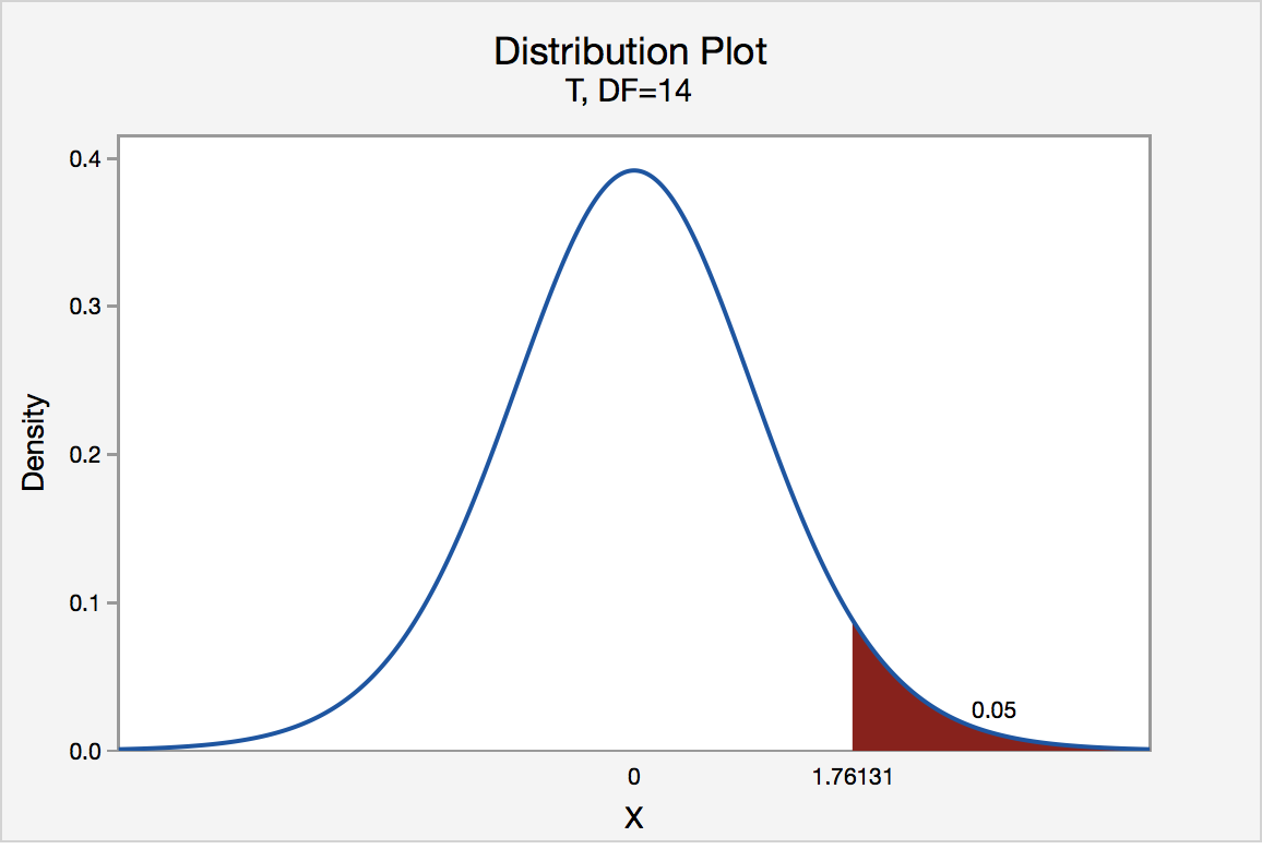
Right-Tailed
The critical value for conducting the right-tailed test H0 : μ = 3 versus HA : μ > 3 is the t-value, denoted t\(\alpha\), n - 1, such that the probability to the right of it is \(\alpha\). It can be shown using either statistical software or a t-table that the critical value t 0.05,14 is 1.7613. That is, we would reject the null hypothesis H0 : μ = 3 in favor of the alternative hypothesis HA : μ > 3 if the test statistic t* is greater than 1.7613. Visually, the rejection region is shaded red in the graph.
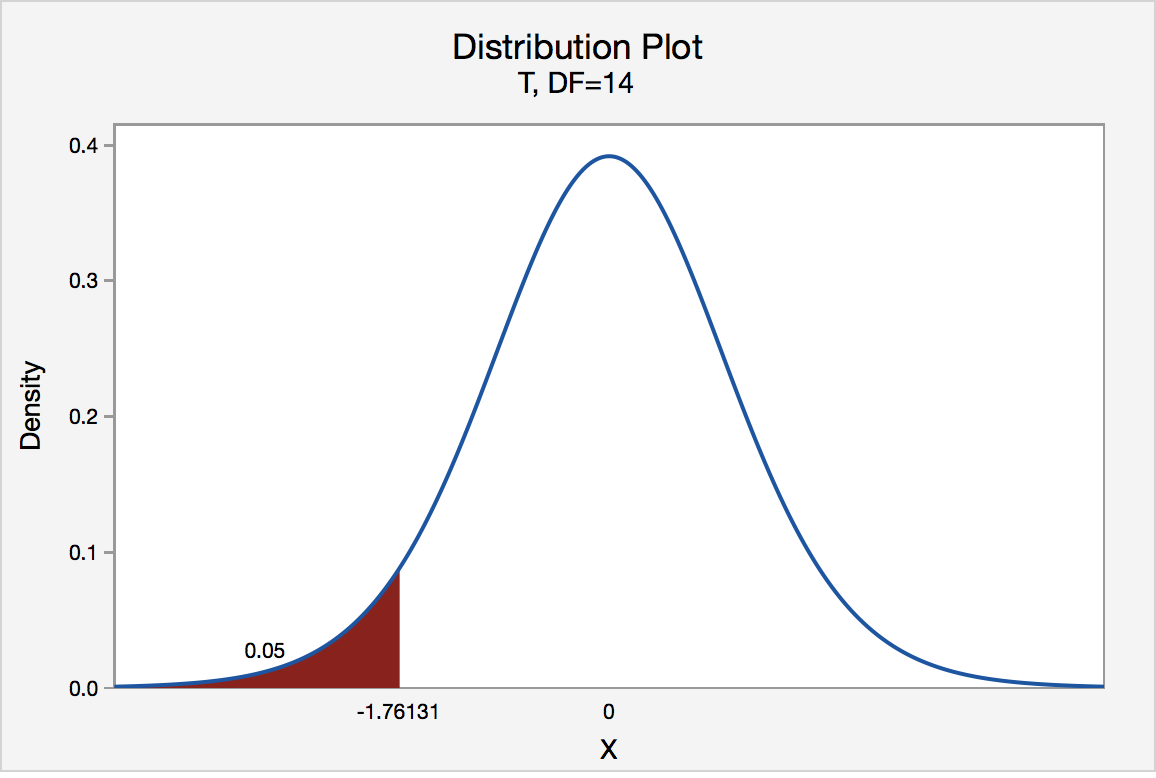
Left-Tailed
The critical value for conducting the left-tailed test H0 : μ = 3 versus HA : μ < 3 is the t-value, denoted -t(\(\alpha\), n - 1), such that the probability to the left of it is \(\alpha\). It can be shown using either statistical software or a t-table that the critical value -t0.05,14 is -1.7613. That is, we would reject the null hypothesis H0 : μ = 3 in favor of the alternative hypothesis HA : μ < 3 if the test statistic t* is less than -1.7613. Visually, the rejection region is shaded red in the graph.
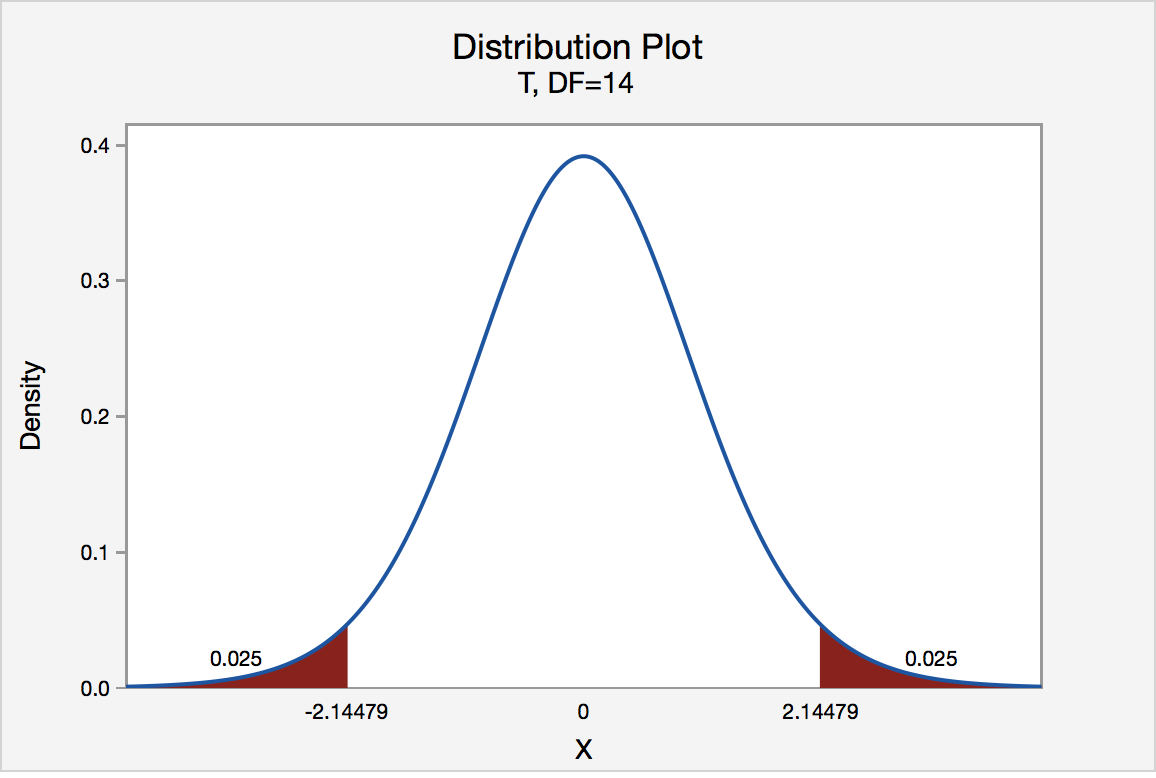
Two-Tailed
There are two critical values for the two-tailed test H0 : μ = 3 versus HA : μ ≠ 3 — one for the left-tail denoted -t(\(\alpha\)/2, n - 1) and one for the right-tail denoted t(\(\alpha\)/2, n - 1). The value -t(\(\alpha\)/2, n - 1) is the t-value such that the probability to the left of it is \(\alpha\)/2, and the value t(\(\alpha\)/2, n - 1) is the t-value such that the probability to the right of it is \(\alpha\)/2. It can be shown using either statistical software or a t-table that the critical value -t0.025,14 is -2.1448 and the critical value t0.025,14 is 2.1448. That is, we would reject the null hypothesis H0 : μ = 3 in favor of the alternative hypothesis HA : μ ≠ 3 if the test statistic t* is less than -2.1448 or greater than 2.1448. Visually, the rejection region is shaded red in the graph.
S.3.2 Hypothesis Testing (P-Value Approach)
S.3.2 Hypothesis Testing (P-Value Approach)The P-value approach involves determining "likely" or "unlikely" by determining the probability — assuming the null hypothesis was true — of observing a more extreme test statistic in the direction of the alternative hypothesis than the one observed. If the P-value is small, say less than (or equal to) \(\alpha\), then it is "unlikely." And, if the P-value is large, say more than \(\alpha\), then it is "likely."
If the P-value is less than (or equal to) \(\alpha\), then the null hypothesis is rejected in favor of the alternative hypothesis. And, if the P-value is greater than \(\alpha\), then the null hypothesis is not rejected.
Specifically, the four steps involved in using the P-value approach to conducting any hypothesis test are:
- Specify the null and alternative hypotheses.
- Using the sample data and assuming the null hypothesis is true, calculate the value of the test statistic. Again, to conduct the hypothesis test for the population mean μ, we use the t-statistic \(t^*=\frac{\bar{x}-\mu}{s/\sqrt{n}}\) which follows a t-distribution with n - 1 degrees of freedom.
- Using the known distribution of the test statistic, calculate the P-value: "If the null hypothesis is true, what is the probability that we'd observe a more extreme test statistic in the direction of the alternative hypothesis than we did?" (Note how this question is equivalent to the question answered in criminal trials: "If the defendant is innocent, what is the chance that we'd observe such extreme criminal evidence?")
- Set the significance level, \(\alpha\), the probability of making a Type I error to be small — 0.01, 0.05, or 0.10. Compare the P-value to \(\alpha\). If the P-value is less than (or equal to) \(\alpha\), reject the null hypothesis in favor of the alternative hypothesis. If the P-value is greater than \(\alpha\), do not reject the null hypothesis.
Example S.3.2.1
Mean GPA
In our example concerning the mean grade point average, suppose that our random sample of n = 15 students majoring in mathematics yields a test statistic t* equaling 2.5. Since n = 15, our test statistic t* has n - 1 = 14 degrees of freedom. Also, suppose we set our significance level α at 0.05 so that we have only a 5% chance of making a Type I error.
Right Tailed
The P-value for conducting the right-tailed test H0 : μ = 3 versus HA : μ > 3 is the probability that we would observe a test statistic greater than t* = 2.5 if the population mean \(\mu\) really were 3. Recall that probability equals the area under the probability curve. The P-value is therefore the area under a tn - 1 = t14 curve and to the right of the test statistic t* = 2.5. It can be shown using statistical software that the P-value is 0.0127. The graph depicts this visually.
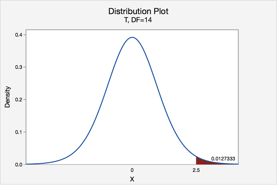
The P-value, 0.0127, tells us it is "unlikely" that we would observe such an extreme test statistic t* in the direction of HA if the null hypothesis were true. Therefore, our initial assumption that the null hypothesis is true must be incorrect. That is, since the P-value, 0.0127, is less than \(\alpha\) = 0.05, we reject the null hypothesis H0 : μ = 3 in favor of the alternative hypothesis HA : μ > 3.
Note that we would not reject H0 : μ = 3 in favor of HA : μ > 3 if we lowered our willingness to make a Type I error to \(\alpha\) = 0.01 instead, as the P-value, 0.0127, is then greater than \(\alpha\) = 0.01.
Left Tailed
In our example concerning the mean grade point average, suppose that our random sample of n = 15 students majoring in mathematics yields a test statistic t* instead of equaling -2.5. The P-value for conducting the left-tailed test H0 : μ = 3 versus HA : μ < 3 is the probability that we would observe a test statistic less than t* = -2.5 if the population mean μ really were 3. The P-value is therefore the area under a tn - 1 = t14 curve and to the left of the test statistic t* = -2.5. It can be shown using statistical software that the P-value is 0.0127. The graph depicts this visually.
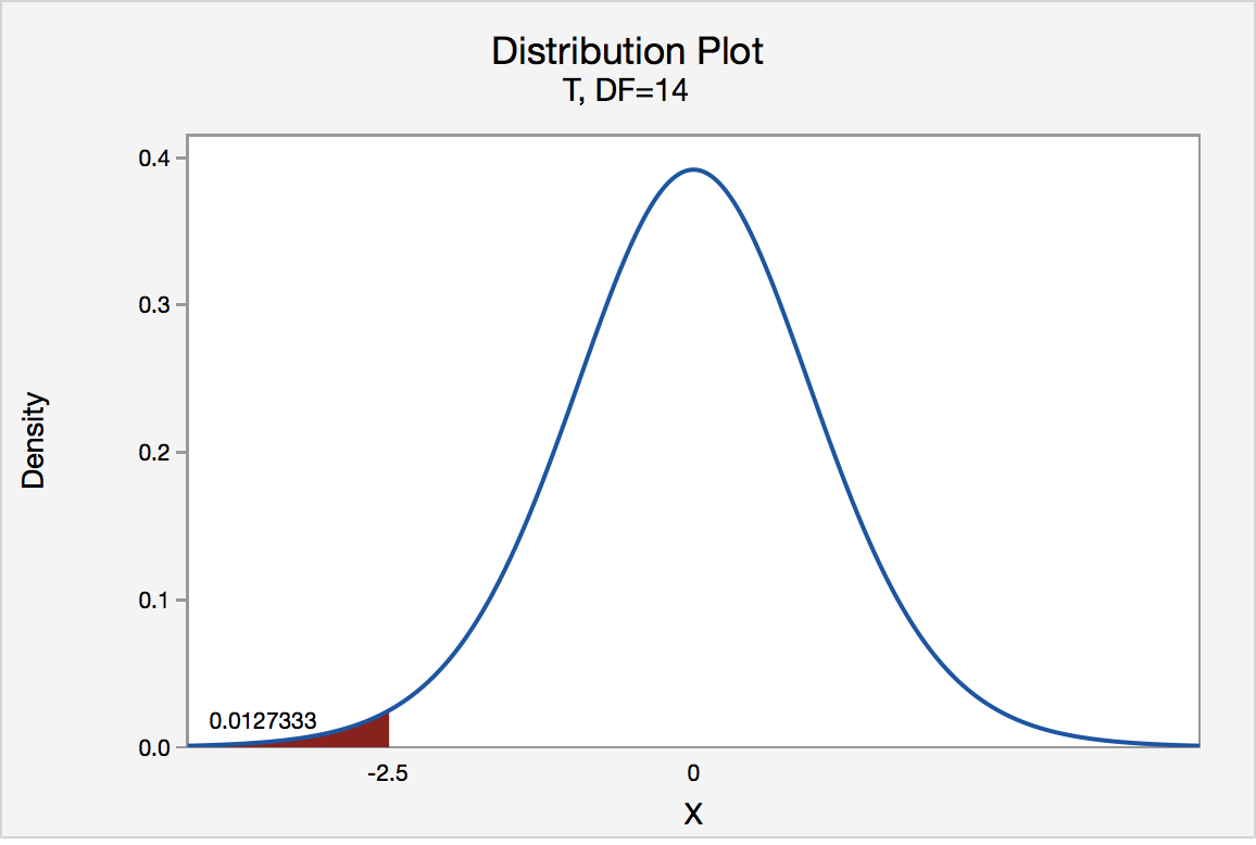
The P-value, 0.0127, tells us it is "unlikely" that we would observe such an extreme test statistic t* in the direction of HA if the null hypothesis were true. Therefore, our initial assumption that the null hypothesis is true must be incorrect. That is, since the P-value, 0.0127, is less than α = 0.05, we reject the null hypothesis H0 : μ = 3 in favor of the alternative hypothesis HA : μ < 3.
Note that we would not reject H0 : μ = 3 in favor of HA : μ < 3 if we lowered our willingness to make a Type I error to α = 0.01 instead, as the P-value, 0.0127, is then greater than \(\alpha\) = 0.01.
Two-Tailed
In our example concerning the mean grade point average, suppose again that our random sample of n = 15 students majoring in mathematics yields a test statistic t* instead of equaling -2.5. The P-value for conducting the two-tailed test H0 : μ = 3 versus HA : μ ≠ 3 is the probability that we would observe a test statistic less than -2.5 or greater than 2.5 if the population mean μ really was 3. That is, the two-tailed test requires taking into account the possibility that the test statistic could fall into either tail (hence the name "two-tailed" test). The P-value is, therefore, the area under a tn - 1 = t14 curve to the left of -2.5 and to the right of 2.5. It can be shown using statistical software that the P-value is 0.0127 + 0.0127, or 0.0254. The graph depicts this visually.
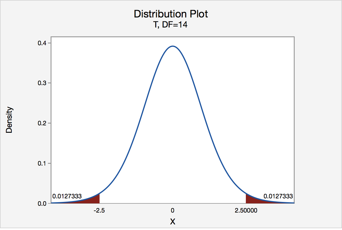
Note that the P-value for a two-tailed test is always two times the P-value for either of the one-tailed tests. The P-value, 0.0254, tells us it is "unlikely" that we would observe such an extreme test statistic t* in the direction of HA if the null hypothesis were true. Therefore, our initial assumption that the null hypothesis is true must be incorrect. That is, since the P-value, 0.0254, is less than α = 0.05, we reject the null hypothesis H0 : μ = 3 in favor of the alternative hypothesis HA : μ ≠ 3.
Note that we would not reject H0 : μ = 3 in favor of HA : μ ≠ 3 if we lowered our willingness to make a Type I error to α = 0.01 instead, as the P-value, 0.0254, is then greater than \(\alpha\) = 0.01.
Now that we have reviewed the critical value and P-value approach procedures for each of the three possible hypotheses, let's look at three new examples — one of a right-tailed test, one of a left-tailed test, and one of a two-tailed test.
The good news is that, whenever possible, we will take advantage of the test statistics and P-values reported in statistical software, such as Minitab, to conduct our hypothesis tests in this course.
S.3.3 Hypothesis Testing Examples
S.3.3 Hypothesis Testing ExamplesBrinell Hardness Scores
An engineer measured the Brinell hardness of 25 pieces of ductile iron that were subcritically annealed. The resulting data were:
| Brinell Hardness of 25 Pieces of Ductile Iron | ||||||||
|---|---|---|---|---|---|---|---|---|
| 170 | 167 | 174 | 179 | 179 | 187 | 179 | 183 | 179 |
| 156 | 163 | 156 | 187 | 156 | 167 | 156 | 174 | 170 |
| 183 | 179 | 174 | 179 | 170 | 159 | 187 | ||
The engineer hypothesized that the mean Brinell hardness of all such ductile iron pieces is greater than 170. Therefore, he was interested in testing the hypotheses:
H0 : μ = 170
HA : μ > 170
The engineer entered his data into Minitab and requested that the "one-sample t-test" be conducted for the above hypotheses. He obtained the following output:
Descriptive Statistics
| N | Mean | StDev | SE Mean | 95% Lower Bound |
|---|---|---|---|---|
| 25 | 172.52 | 10.31 | 2.06 | 168.99 |
$\mu$: mean of Brinelli
Test
Null hypothesis H₀: $\mu$ = 170
Alternative hypothesis H₁: $\mu$ > 170
| T-Value | P-Value |
|---|---|
| 1.22 | 0.117 |
The output tells us that the average Brinell hardness of the n = 25 pieces of ductile iron was 172.52 with a standard deviation of 10.31. (The standard error of the mean "SE Mean", calculated by dividing the standard deviation 10.31 by the square root of n = 25, is 2.06). The test statistic t* is 1.22, and the P-value is 0.117.
If the engineer set his significance level α at 0.05 and used the critical value approach to conduct his hypothesis test, he would reject the null hypothesis if his test statistic t* were greater than 1.7109 (determined using statistical software or a t-table):
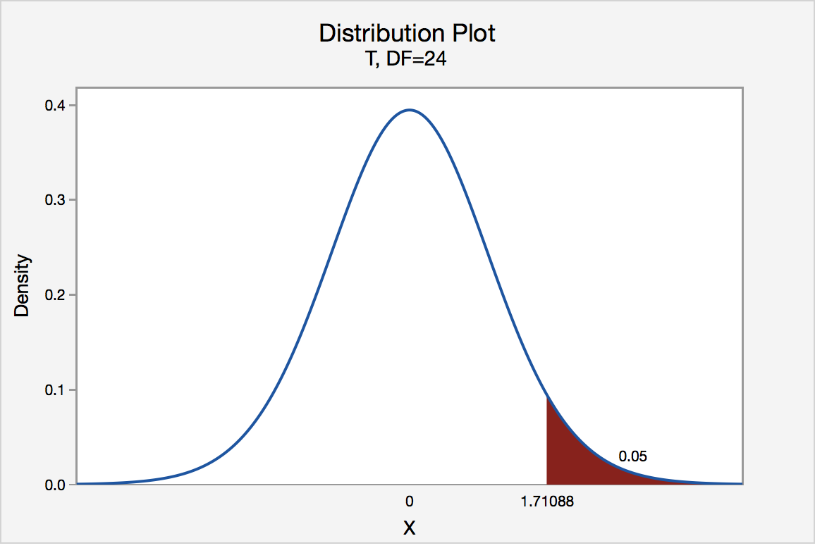
Since the engineer's test statistic, t* = 1.22, is not greater than 1.7109, the engineer fails to reject the null hypothesis. That is, the test statistic does not fall in the "critical region." There is insufficient evidence, at the \(\alpha\) = 0.05 level, to conclude that the mean Brinell hardness of all such ductile iron pieces is greater than 170.
If the engineer used the P-value approach to conduct his hypothesis test, he would determine the area under a tn - 1 = t24 curve and to the right of the test statistic t* = 1.22:
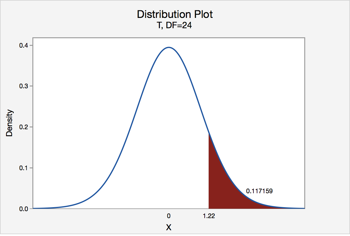
In the output above, Minitab reports that the P-value is 0.117. Since the P-value, 0.117, is greater than \(\alpha\) = 0.05, the engineer fails to reject the null hypothesis. There is insufficient evidence, at the \(\alpha\) = 0.05 level, to conclude that the mean Brinell hardness of all such ductile iron pieces is greater than 170.
Note that the engineer obtains the same scientific conclusion regardless of the approach used. This will always be the case.
Height of Sunflowers
A biologist was interested in determining whether sunflower seedlings treated with an extract from Vinca minor roots resulted in a lower average height of sunflower seedlings than the standard height of 15.7 cm. The biologist treated a random sample of n = 33 seedlings with the extract and subsequently obtained the following heights:
| Heights of 33 Sunflower Seedlings | ||||||||
|---|---|---|---|---|---|---|---|---|
| 11.5 | 11.8 | 15.7 | 16.1 | 14.1 | 10.5 | 9.3 | 15.0 | 11.1 |
| 15.2 | 19.0 | 12.8 | 12.4 | 19.2 | 13.5 | 12.2 | 13.3 | |
| 16.5 | 13.5 | 14.4 | 16.7 | 10.9 | 13.0 | 10.3 | 15.8 | |
| 15.1 | 17.1 | 13.3 | 12.4 | 8.5 | 14.3 | 12.9 | 13.5 | |
The biologist's hypotheses are:
H0 : μ = 15.7
HA : μ < 15.7
The biologist entered her data into Minitab and requested that the "one-sample t-test" be conducted for the above hypotheses. She obtained the following output:
Descriptive Statistics
| N | Mean | StDev | SE Mean | 95% Upper Bound |
|---|---|---|---|---|
| 33 | 13.664 | 2.544 | 0.443 | 14.414 |
$\mu$: mean of Height
Test
Null hypothesis H₀: $\mu$ = 15.7
Alternative hypothesis H₁: $\mu$ < 15.7
| T-Value | P-Value |
|---|---|
| -4.60 | 0.000 |
The output tells us that the average height of the n = 33 sunflower seedlings was 13.664 with a standard deviation of 2.544. (The standard error of the mean "SE Mean", calculated by dividing the standard deviation 13.664 by the square root of n = 33, is 0.443). The test statistic t* is -4.60, and the P-value, 0.000, is to three decimal places.
Minitab Note. Minitab will always report P-values to only 3 decimal places. If Minitab reports the P-value as 0.000, it really means that the P-value is 0.000....something. Throughout this course (and your future research!), when you see that Minitab reports the P-value as 0.000, you should report the P-value as being "< 0.001."
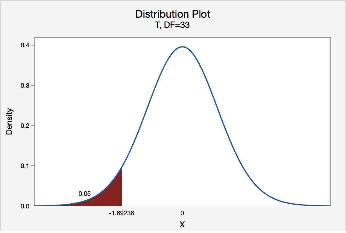
If the biologist set her significance level \(\alpha\) at 0.05 and used the critical value approach to conduct her hypothesis test, she would reject the null hypothesis if her test statistic t* were less than -1.6939 (determined using statistical software or a t-table):s-3-3
Since the biologist's test statistic, t* = -4.60, is less than -1.6939, the biologist rejects the null hypothesis. That is, the test statistic falls in the "critical region." There is sufficient evidence, at the α = 0.05 level, to conclude that the mean height of all such sunflower seedlings is less than 15.7 cm.
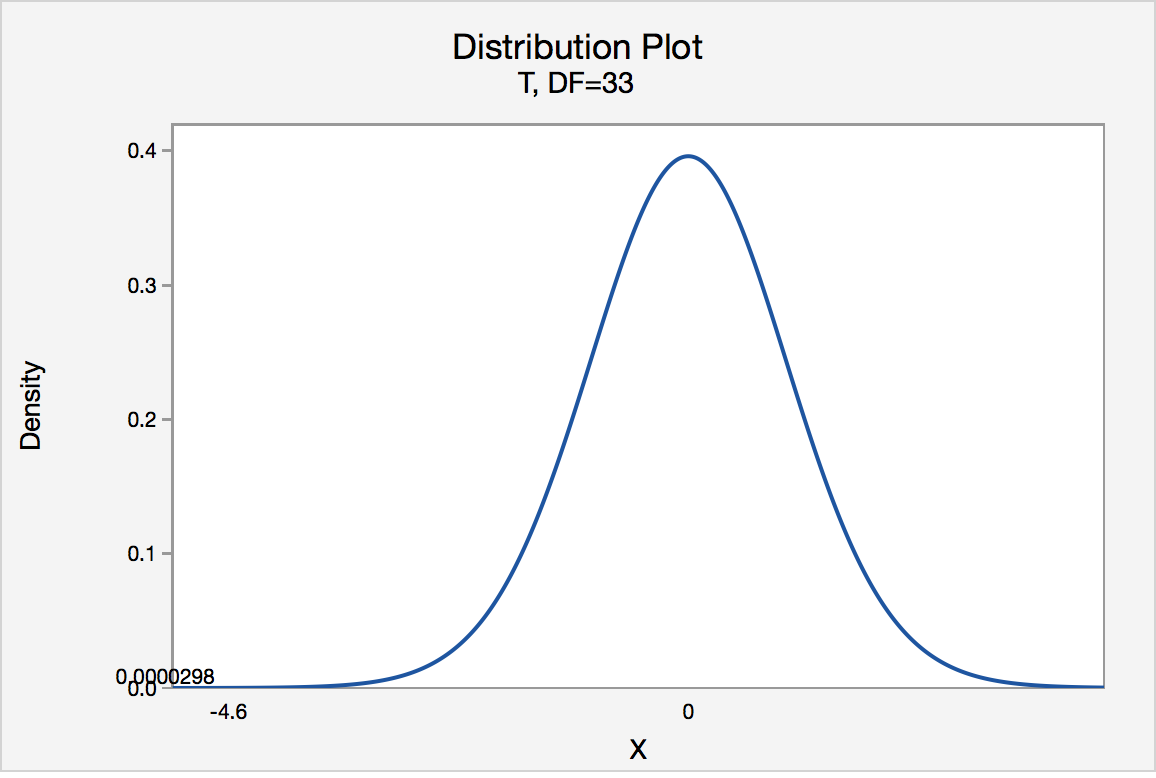
If the biologist used the P-value approach to conduct her hypothesis test, she would determine the area under a tn - 1 = t32 curve and to the left of the test statistic t* = -4.60:
In the output above, Minitab reports that the P-value is 0.000, which we take to mean < 0.001. Since the P-value is less than 0.001, it is clearly less than \(\alpha\) = 0.05, and the biologist rejects the null hypothesis. There is sufficient evidence, at the \(\alpha\) = 0.05 level, to conclude that the mean height of all such sunflower seedlings is less than 15.7 cm.
Note again that the biologist obtains the same scientific conclusion regardless of the approach used. This will always be the case.
Gum Thickness
A manufacturer claims that the thickness of the spearmint gum it produces is 7.5 one-hundredths of an inch. A quality control specialist regularly checks this claim. On one production run, he took a random sample of n = 10 pieces of gum and measured their thickness. He obtained:
| Thicknesses of 10 Pieces of Gum | ||||
|---|---|---|---|---|
| 7.65 | 7.60 | 7.65 | 7.70 | 7.55 |
| 7.55 | 7.40 | 7.40 | 7.50 | 7.50 |
The quality control specialist's hypotheses are:
H0 : μ = 7.5
HA : μ ≠ 7.5
The quality control specialist entered his data into Minitab and requested that the "one-sample t-test" be conducted for the above hypotheses. He obtained the following output:
Descriptive Statistics
| N | Mean | StDev | SE Mean | 95% CI for $\mu$ |
|---|---|---|---|---|
| 10 | 7.550 | 0.1027 | 0.0325 | (7.4765, 7.6235) |
$\mu$: mean of Thickness
Test
Null hypothesis H₀: $\mu$ = 7.5
Alternative hypothesis H₁: $\mu \ne$ 7.5
| T-Value | P-Value |
|---|---|
| 1.54 | 0.158 |
The output tells us that the average thickness of the n = 10 pieces of gums was 7.55 one-hundredths of an inch with a standard deviation of 0.1027. (The standard error of the mean "SE Mean", calculated by dividing the standard deviation 0.1027 by the square root of n = 10, is 0.0325). The test statistic t* is 1.54, and the P-value is 0.158.
If the quality control specialist sets his significance level \(\alpha\) at 0.05 and used the critical value approach to conduct his hypothesis test, he would reject the null hypothesis if his test statistic t* were less than -2.2616 or greater than 2.2616 (determined using statistical software or a t-table):
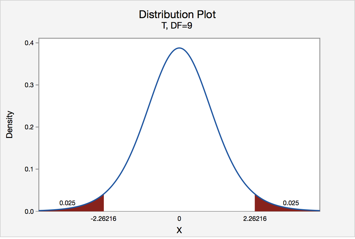
Since the quality control specialist's test statistic, t* = 1.54, is not less than -2.2616 nor greater than 2.2616, the quality control specialist fails to reject the null hypothesis. That is, the test statistic does not fall in the "critical region." There is insufficient evidence, at the \(\alpha\) = 0.05 level, to conclude that the mean thickness of all of the manufacturer's spearmint gum differs from 7.5 one-hundredths of an inch.
If the quality control specialist used the P-value approach to conduct his hypothesis test, he would determine the area under a tn - 1 = t9 curve, to the right of 1.54 and to the left of -1.54:
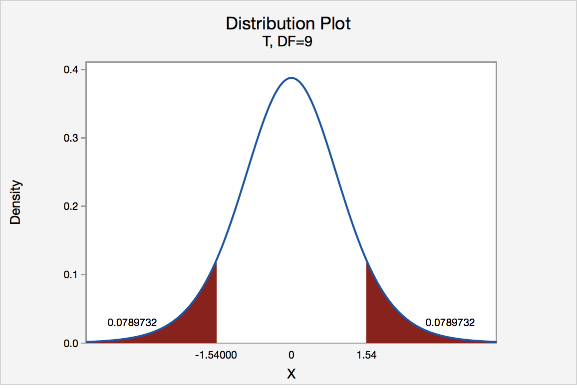
In the output above, Minitab reports that the P-value is 0.158. Since the P-value, 0.158, is greater than \(\alpha\) = 0.05, the quality control specialist fails to reject the null hypothesis. There is insufficient evidence, at the \(\alpha\) = 0.05 level, to conclude that the mean thickness of all pieces of spearmint gum differs from 7.5 one-hundredths of an inch.
Note that the quality control specialist obtains the same scientific conclusion regardless of the approach used. This will always be the case.
In closing
In our review of hypothesis tests, we have focused on just one particular hypothesis test, namely that concerning the population mean \(\mu\). The important thing to recognize is that the topics discussed here — the general idea of hypothesis tests, errors in hypothesis testing, the critical value approach, and the P-value approach — generally extend to all of the hypothesis tests you will encounter.
S.4 Chi-Square Tests
S.4 Chi-Square TestsChi-Square Test of Independence
Do you remember how to test the independence of two categorical variables? This test is performed by using a Chi-square test of independence.
Recall that we can summarize two categorical variables within a two-way table, also called an r × c contingency table, where r = number of rows, c = number of columns. Our question of interest is “Are the two variables independent?” This question is set up using the following hypothesis statements:
- Null Hypothesis
- The two categorical variables are independent
- Alternative Hypothesis
- The two categorical variables are dependent
- Chi-Square Test Statistic
- \(\chi^2=\sum(O-E)^2/E\)
- where O represents the observed frequency. E is the expected frequency under the null hypothesis and computed by:
\[E=\frac{\text{row total}\times\text{column total}}{\text{sample size}}\]
We will compare the value of the test statistic to the critical value of \(\chi_{\alpha}^2\) with the degree of freedom = (r - 1) (c - 1), and reject the null hypothesis if \(\chi^2 \gt \chi_{\alpha}^2\).
Example S.4.1
Is gender independent of education level? A random sample of 395 people was surveyed and each person was asked to report the highest education level they obtained. The data that resulted from the survey are summarized in the following table:
| High School | Bachelors | Masters | Ph.d. | Total | |
|---|---|---|---|---|---|
| Female | 60 | 54 | 46 | 41 | 201 |
| Male | 40 | 44 | 53 | 57 | 194 |
| Total | 100 | 98 | 99 | 98 | 395 |
Question: Are gender and education level dependent at a 5% level of significance? In other words, given the data collected above, is there a relationship between the gender of an individual and the level of education that they have obtained?
Here's the table of expected counts:
| High School | Bachelors | Masters | Ph.d. | Total | |
|---|---|---|---|---|---|
| Female | 50.886 | 49.868 | 50.377 | 49.868 | 201 |
| Male | 49.114 | 48.132 | 48.623 | 48.132 | 194 |
| Total | 100 | 98 | 99 | 98 | 395 |
So, working this out, \(\chi^2= \dfrac{(60−50.886)^2}{50.886} + \cdots + \dfrac{(57 − 48.132)^2}{48.132} = 8.006\)
The critical value of \(\chi^2\) with 3 degrees of freedom is 7.815. Since 8.006 > 7.815, we reject the null hypothesis and conclude that the education level depends on gender at a 5% level of significance.
S.5 Power Analysis
S.5 Power AnalysisWhy is Power Analysis Important?
Consider a research experiment where the p-value computed from the data was 0.12. As a result, one would fail to reject the null hypothesis because this p-value is larger than \(\alpha\) = 0.05. However, there still exist two possible cases for which we failed to reject the null hypothesis:
- the null hypothesis is a reasonable conclusion,
- the sample size is not large enough to either accept or reject the null hypothesis, i.e., additional samples might provide additional evidence.
Power analysis is the procedure that researchers can use to determine if the test contains enough power to make a reasonable conclusion. From another perspective power analysis can also be used to calculate the number of samples required to achieve a specified level of power.
Example S.5.1
Let's take a look at an example that illustrates how to compute the power of the test.
Example
Let X denote the height of randomly selected Penn State students. Assume that X is normally distributed with unknown mean \(\mu\) and a standard deviation of 9. Take a random sample of n = 25 students, so that, after setting the probability of committing a Type I error at \(\alpha = 0.05\), we can test the null hypothesis \(H_0: \mu = 170\) against the alternative hypothesis that \(H_A: \mu > 170\).
What is the power of the hypothesis test if the true population mean were \(\mu = 175\)?
\[\begin{align}z&=\frac{\bar{x}-\mu}{\sigma / \sqrt{n}} \\
\bar{x}&= \mu + z \left(\frac{\sigma}{\sqrt{n}}\right) \\
\bar{x}&=170+1.645\left(\frac{9}{\sqrt{25}}\right) \\
&=172.961\\
\end{align}\]
So we should reject the null hypothesis when the observed sample mean is 172.961 or greater:
We get
\[\begin{align}\text{Power}&=P(\bar{x} \ge 172.961 \text{ when } \mu =175)\\
&=P\left(z \ge \frac{172.961-175}{9/\sqrt{25}} \right)\\
&=P(z \ge -1.133)\\
&= 0.8713\\
\end{align}\]
and illustrated below:
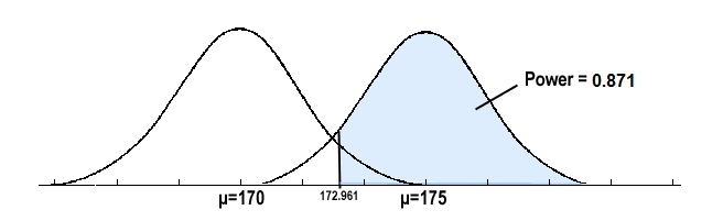
In summary, we have determined that we have an 87.13% chance of rejecting the null hypothesis \(H_0: \mu = 170\) in favor of the alternative hypothesis \(H_A: \mu > 170\) if the true unknown population mean is, in reality, \(\mu = 175\).
Calculating Sample Size
If the sample size is fixed, then decreasing Type I error \(\alpha\) will increase Type II error \(\beta\). If one wants both to decrease, then one has to increase the sample size.
To calculate the smallest sample size needed for specified \(\alpha\), \(\beta\), \(\mu_a\), then (\(\mu_a\) is the likely value of \(\mu\) at which you want to evaluate the power.
- Sample Size for One-Tailed Test
- \(n = \dfrac{\sigma^2(Z_{\alpha}+Z_{\beta})^2}{(\mu_0−\mu_a)^2}\)
- Sample Size for Two-Tailed Test
- \(n = \dfrac{\sigma^2(Z_{\alpha/2}+Z_{\beta})^2}{(\mu_0−\mu_a)^2}\)
Let's investigate by returning to our previous example.
Example S.5.2
Let X denote the height of randomly selected Penn State students. Assume that X is normally distributed with unknown mean \(\mu\) and standard deviation 9. We are interested in testing at \(\alpha = 0.05\) level , the null hypothesis \(H_0: \mu = 170\) against the alternative hypothesis that \(H_A: \mu > 170\).
Find the sample size n that is necessary to achieve 0.90 power at the alternative μ = 175.
\[\begin{align}n&= \dfrac{\sigma^2(Z_{\alpha}+Z_{\beta})^2}{(\mu_0−\mu_a)^2}\\ &=\dfrac{9^2 (1.645 + 1.28)^2}{(170-175)^2}\\ &=27.72\\ n&=28\\ \end{align}\]
In summary, you should see how power analysis is very important so that we are able to make the correct decision when the data indicate that one cannot reject the null hypothesis. You should also see how power analysis can also be used to calculate the minimum sample size required to detect a difference that meets the needs of your research.
S.6 Test of Proportion
S.6 Test of ProportionLet us consider the parameter p of the population proportion. For instance, we might want to know the proportion of males within a total population of adults when we conduct a survey. A test of proportion will assess whether or not a sample from a population represents the true proportion of the entire population.
Critical Value Approach
The steps to perform a test of proportion using the critical value approval are as follows:
- State the null hypothesis H0 and the alternative hypothesis HA.
- Calculate the test statistic:
\[z=\frac{\hat{p}-p_0}{\sqrt{\frac{p_0(1-p_0)}{n}}}\]
where \(p_0\) is the null hypothesized proportion i.e., when \(H_0: p=p_0\)
-
Determine the critical region.
-
Make a decision. Determine if the test statistic falls in the critical region. If it does, reject the null hypothesis. If it does not, do not reject the null hypothesis.
Example S.6.1
Newborn babies are more likely to be boys than girls. A random sample found 13,173 boys were born among 25,468 newborn children. The sample proportion of boys was 0.5172. Is this sample evidence that the birth of boys is more common than the birth of girls in the entire population?
Here, we want to test
\(H_0: p=0.5\)
\(H_A: p>0.5\)
The test statistic
\[\begin{align} z &=\frac{\hat{p}-p_o}{\sqrt{\frac{p_0(1-p_0)}{n}}}\\
&=\frac{0.5172-0.5}{\sqrt{\frac{0.5(1-0.5)}{25468}}}\\
&= 5.49 \end{align}\]
We will reject the null hypothesis \(H_0: p = 0.5\) if \(\hat{p} > 0.5052\) or equivalently if Z > 1.645
Here's a picture of such a "critical region" (or "rejection region"):
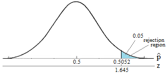
It looks like we should reject the null hypothesis because:
\[\hat{p}= 0.5172 > 0.5052\]
or equivalently since our test statistic Z = 5.49 is greater than 1.645.
Our Conclusion: We say there is sufficient evidence to conclude boys are more common than girls in the entire population.
\(p\)- value Approach
Next, let's state the procedure in terms of performing a proportion test using the p-value approach. The basic procedure is:
- State the null hypothesis H0 and the alternative hypothesis HA.
- Set the level of significance \(\alpha\).
- Calculate the test statistic:
\[z=\frac{\hat{p}-p_o}{\sqrt{\frac{p_0(1-p_0)}{n}}}\]
-
Calculate the p-value.
-
Make a decision. Check whether to reject the null hypothesis by comparing the p-value to \(\alpha\). If the p-value < \(\alpha\) then reject \(H_0\); otherwise do not reject \(H_0\).
Example S.6.2
Let's investigate by returning to our previous example. Again, we want to test
\(H_0: p=0.5\)
\(H_A: p>0.5\)
The test statistic
\[\begin{align} z &=\frac{\hat{p}-p_o}{\sqrt{\frac{p_0(1-p_0)}{n}}}\\
&=\frac{0.5172-0.5}{\sqrt{\frac{0.5(1-0.5)}{25468}}}\\
&= 5.49 \end{align}\]
The p-value is represented in the graph below:
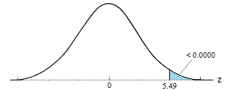
\[P = P(Z \ge 5.49) = 0.0000 \cdots \doteq 0\]
Our Conclusion: Because the p-value is smaller than the significance level \(\alpha = 0.05\), we can reject the null hypothesis. Again, we would say that there is sufficient evidence to conclude boys are more common than girls in the entire population at the \(\alpha = 0.05\) level.
As should always be the case, the two approaches, the critical value approach and the p-value approach lead to the same conclusion.
S.7 Self-Assess
S.7 Self-AssessWe suggest you...
- Review the concepts and methods on the pages in this section of this website.
- Download and Complete the Self-Assessment Exam.
- Determine your Score by reviewing the Self-Assessment Exam Solutions
A score below 70% suggests that the concepts and procedures that are covered in STAT 500 have not been mastered adequately. Students are strongly encouraged to take STAT 500, thoroughly review the materials that are covered in the sections above or take additional coursework that focuses on these foundations.
If you have struggled with the concepts and methods that are presented here, you will indeed struggle in any of the graduate-level courses included in the Master of Applied Statistics program above STAT 500 that expect and build on this foundation.
Note: These materials are NOT intended to be a complete treatment of the ideas and methods used in basic statistics. These materials and the accompanying self-assessment are simply intended as simply an 'early warning signal' for students. Also, please note that completing the self-assessment successfully does not automatically ensure success in any of the courses that use this foundation.