S.3 Hypothesis Testing

In reviewing hypothesis tests, we start first with the general idea. Then, we keep returning to the basic procedures of hypothesis testing, each time adding a little more detail.

The general idea of hypothesis testing involves:

Making an initial assumption.
Collecting evidence (data).
Based on the available evidence (data), deciding whether to reject or not reject the initial assumption.

Every hypothesis test — regardless of the population parameter involved — requires the above three steps.

Example S.3.1

Is Normal Body Temperature Really 98.6 Degrees F?

Consider the population of many, many adults. A researcher hypothesized that the average adult body temperature is lower than the often-advertised 98.6 degrees F. That is, the researcher wants an answer to the question: "Is the average adult body temperature 98.6 degrees? Or is it lower?" To answer his research question, the researcher starts by assuming that the average adult body temperature was 98.6 degrees F.

Then, the researcher went out and tried to find evidence that refutes his initial assumption. In doing so, he selects a random sample of 130 adults. The average body temperature of the 130 sampled adults is 98.25 degrees.

Then, the researcher uses the data he collected to make a decision about his initial assumption. It is either likely or unlikely that the researcher would collect the evidence he did given his initial assumption that the average adult body temperature is 98.6 degrees:

If it is likely, then the researcher does not reject his initial assumption that the average adult body temperature is 98.6 degrees. There is not enough evidence to do otherwise.
If it is unlikely, then:
- either the researcher's initial assumption is correct and he experienced a very unusual event;
- or the researcher's initial assumption is incorrect.

In statistics, we generally don't make claims that require us to believe that a very unusual event happened. That is, in the practice of statistics, if the evidence (data) we collected is unlikely in light of the initial assumption, then we reject our initial assumption.

Example S.3.2

Criminal Trial Analogy

One place where you can consistently see the general idea of hypothesis testing in action is in criminal trials held in the United States. Our criminal justice system assumes "the defendant is innocent until proven guilty." That is, our initial assumption is that the defendant is innocent.

In the practice of statistics, we make our initial assumption when we state our two competing hypotheses -- the null hypothesis (H₀) and the alternative hypothesis (H_A). Here, our hypotheses are:

H₀: Defendant is not guilty (innocent)
H_A: Defendant is guilty

In statistics, we always assume the null hypothesis is true. That is, the null hypothesis is always our initial assumption.

The prosecution team then collects evidence — such as finger prints, blood spots, hair samples, carpet fibers, shoe prints, ransom notes, and handwriting samples — with the hopes of finding "sufficient evidence" to make the assumption of innocence refutable.

In statistics, the data are the evidence.

The jury then makes a decision based on the available evidence:

If the jury finds sufficient evidence — beyond a reasonable doubt — to make the assumption of innocence refutable, the jury rejects the null hypothesis and deems the defendant guilty. We behave as if the defendant is guilty.
If there is insufficient evidence, then the jury does not reject the null hypothesis. We behave as if the defendant is innocent.

In statistics, we always make one of two decisions. We either "reject the null hypothesis" or we "fail to reject the null hypothesis."

Errors in Hypothesis Testing

Did you notice the use of the phrase "behave as if" in the previous discussion? We "behave as if" the defendant is guilty; we do not "prove" that the defendant is guilty. And, we "behave as if" the defendant is innocent; we do not "prove" that the defendant is innocent.

This is a very important distinction! We make our decision based on evidence not on 100% guaranteed proof. Again:

If we reject the null hypothesis, we do not prove that the alternative hypothesis is true.
If we do not reject the null hypothesis, we do not prove that the null hypothesis is true.

We merely state that there is enough evidence to behave one way or the other. This is always true in statistics! Because of this, whatever the decision, there is always a chance that we made an error.

Let's review the two types of errors that can be made in criminal trials:

Table S.3.1
Truth
	Not Guilty	Guilty
Not Guilty	OK	ERROR
Guilty	ERROR	OK

Table S.3.2 shows how this corresponds to the two types of errors in hypothesis testing.

Table S.3.2
Truth
	Null Hypothesis	Alternative Hypothesis
Do not Reject Null	OK	Type II Error
Reject Null	Type I Error	OK

Note that, in statistics, we call the two types of errors by two different names -- one is called a "Type I error," and the other is called a "Type II error." Here are the formal definitions of the two types of errors:

Type I Error: The null hypothesis is rejected when it is true.

Type II Error: The null hypothesis is not rejected when it is false.

There is always a chance of making one of these errors. But, a good scientific study will minimize the chance of doing so!

Making the Decision

Recall that it is either likely or unlikely that we would observe the evidence we did given our initial assumption. If it is likely, we do not reject the null hypothesis. If it is unlikely, then we reject the null hypothesis in favor of the alternative hypothesis. Effectively, then, making the decision reduces to determining "likely" or "unlikely."

In statistics, there are two ways to determine whether the evidence is likely or unlikely given the initial assumption:

We could take the "critical value approach" (favored in many of the older textbooks).
Or, we could take the "P-value approach" (what is used most often in research, journal articles, and statistical software).

In the next two sections, we review the procedures behind each of these two approaches. To make our review concrete, let's imagine that μ is the average grade point average of all American students who major in mathematics. We first review the critical value approach for conducting each of the following three hypothesis tests about the population mean $\mu$:

Type	Null	Alternative
Right-tailed	H₀ : μ = 3	H_A : μ > 3
Left-tailed	H₀ : μ = 3	H_A : μ < 3
Two-tailed	H₀ : μ = 3	H_A : μ ≠ 3

In Practice

We would want to conduct the first hypothesis test if we were interested in concluding that the average grade point average of the group is more than 3.
We would want to conduct the second hypothesis test if we were interested in concluding that the average grade point average of the group is less than 3.
And, we would want to conduct the third hypothesis test if we were only interested in concluding that the average grade point average of the group differs from 3 (without caring whether it is more or less than 3).

Upon completing the review of the critical value approach, we review the P-value approach for conducting each of the above three hypothesis tests about the population mean $\mu$. The procedures that we review here for both approaches easily extend to hypothesis tests about any other population parameter.

S.3.1 Hypothesis Testing (Critical Value Approach)

The critical value approach involves determining "likely" or "unlikely" by determining whether or not the observed test statistic is more extreme than would be expected if the null hypothesis were true. That is, it entails comparing the observed test statistic to some cutoff value, called the "critical value." If the test statistic is more extreme than the critical value, then the null hypothesis is rejected in favor of the alternative hypothesis. If the test statistic is not as extreme as the critical value, then the null hypothesis is not rejected.

Specifically, the four steps involved in using the critical value approach to conducting any hypothesis test are:

Specify the null and alternative hypotheses.
Using the sample data and assuming the null hypothesis is true, calculate the value of the test statistic. To conduct the hypothesis test for the population mean μ, we use the t-statistic $t^*=\frac{\bar{x}-\mu}{s/\sqrt{n}}$ which follows a t-distribution with n - 1 degrees of freedom.
Determine the critical value by finding the value of the known distribution of the test statistic such that the probability of making a Type I error — which is denoted $\alpha$ (greek letter "alpha") and is called the "significance level of the test" — is small (typically 0.01, 0.05, or 0.10).
Compare the test statistic to the critical value. If the test statistic is more extreme in the direction of the alternative than the critical value, reject the null hypothesis in favor of the alternative hypothesis. If the test statistic is less extreme than the critical value, do not reject the null hypothesis.

Example S.3.1.1

Mean GPA

In our example concerning the mean grade point average, suppose we take a random sample of n = 15 students majoring in mathematics. Since n = 15, our test statistic t* has n - 1 = 14 degrees of freedom. Also, suppose we set our significance level α at 0.05 so that we have only a 5% chance of making a Type I error.

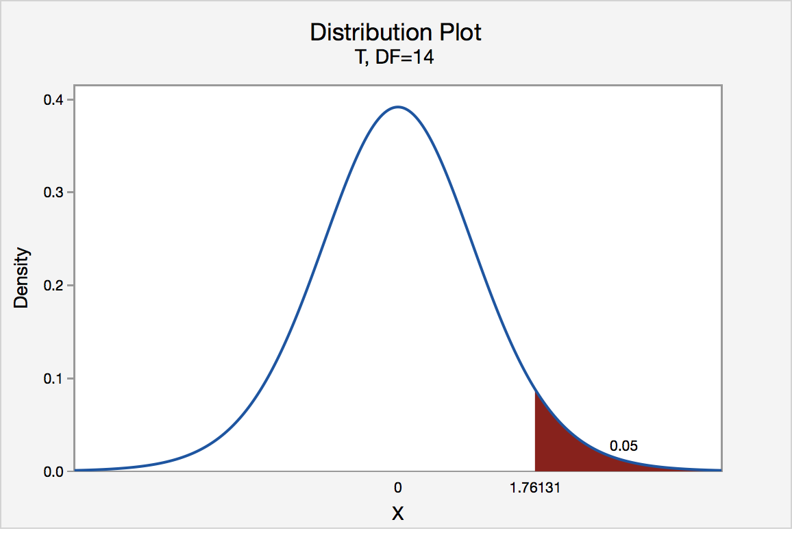
Right-Tailed

The critical value for conducting the right-tailed test H₀ : μ = 3 versus H_A : μ > 3 is the t-value, denoted t_$\alpha$, n - 1, such that the probability to the right of it is $\alpha$. It can be shown using either statistical software or a t-table that the critical value t _0.05,14 is 1.7613. That is, we would reject the null hypothesis H₀ : μ = 3 in favor of the alternative hypothesis H_A : μ > 3 if the test statistic t* is greater than 1.7613. Visually, the rejection region is shaded red in the graph.

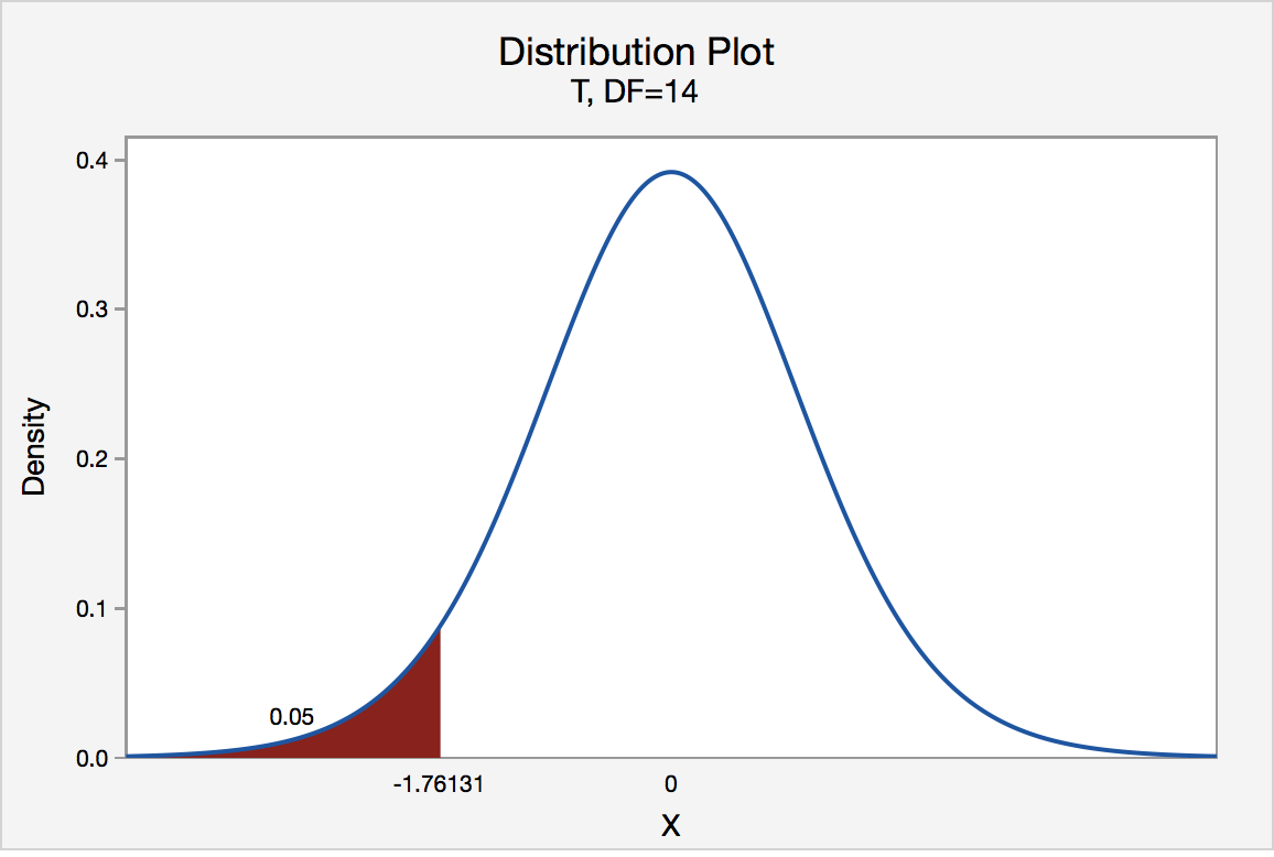
t distribution graph for a t value of 1.76131

Left-Tailed

The critical value for conducting the left-tailed test H₀ : μ = 3 versus H_A : μ < 3 is the t-value, denoted -t_{($\alpha$, n - 1)}, such that the probability to the left of it is $\alpha$. It can be shown using either statistical software or a t-table that the critical value -t_0.05,14 is -1.7613. That is, we would reject the null hypothesis H₀ : μ = 3 in favor of the alternative hypothesis H_A : μ < 3 if the test statistic t* is less than -1.7613. Visually, the rejection region is shaded red in the graph.

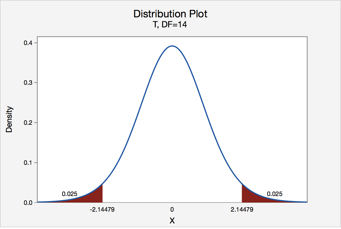
Two-Tailed

There are two critical values for the two-tailed test H₀ : μ = 3 versus H_A : μ ≠ 3 — one for the left-tail denoted -t_{($\alpha$_/2, n - 1)}and one for the right-tail denoted t_{($\alpha$_/2, n - 1)}. The value -t_{($\alpha$/2, n - 1)} is the t-value such that the probability to the left of it is $\alpha$/2, and the value t_{($\alpha$/2, n - 1)} is the t-value such that the probability to the right of it is $\alpha$/2. It can be shown using either statistical software or a t-table that the critical value -t_0.025,14 is -2.1448 and the critical value t_0.025,14 is 2.1448. That is, we would reject the null hypothesis H₀ : μ = 3 in favor of the alternative hypothesis H_A : μ ≠ 3 if the test statistic t* is less than -2.1448 or greater than 2.1448. Visually, the rejection region is shaded red in the graph.

S.3.2 Hypothesis Testing (P-Value Approach)

The P-value approach involves determining "likely" or "unlikely" by determining the probability — assuming the null hypothesis was true — of observing a more extreme test statistic in the direction of the alternative hypothesis than the one observed. If the P-value is small, say less than (or equal to) $\alpha$, then it is "unlikely." And, if the P-value is large, say more than $\alpha$, then it is "likely."

If the P-value is less than (or equal to) $\alpha$, then the null hypothesis is rejected in favor of the alternative hypothesis. And, if the P-value is greater than $\alpha$, then the null hypothesis is not rejected.

Specifically, the four steps involved in using the P-value approach to conducting any hypothesis test are:

Specify the null and alternative hypotheses.
Using the sample data and assuming the null hypothesis is true, calculate the value of the test statistic. Again, to conduct the hypothesis test for the population mean μ, we use the t-statistic $t^*=\frac{\bar{x}-\mu}{s/\sqrt{n}}$ which follows a t-distribution with n - 1 degrees of freedom.
Using the known distribution of the test statistic, calculate the P-value: "If the null hypothesis is true, what is the probability that we'd observe a more extreme test statistic in the direction of the alternative hypothesis than we did?" (Note how this question is equivalent to the question answered in criminal trials: "If the defendant is innocent, what is the chance that we'd observe such extreme criminal evidence?")
Set the significance level, $\alpha$, the probability of making a Type I error to be small — 0.01, 0.05, or 0.10. Compare the P-value to $\alpha$. If the P-value is less than (or equal to) $\alpha$, reject the null hypothesis in favor of the alternative hypothesis. If the P-value is greater than $\alpha$, do not reject the null hypothesis.

Example S.3.2.1

Mean GPA

In our example concerning the mean grade point average, suppose that our random sample of n = 15 students majoring in mathematics yields a test statistic t* equaling 2.5. Since n = 15, our test statistic t* has n - 1 = 14 degrees of freedom. Also, suppose we set our significance level α at 0.05 so that we have only a 5% chance of making a Type I error.

Right Tailed

The P-value for conducting the right-tailed test H₀ : μ = 3 versus H_A : μ > 3 is the probability that we would observe a test statistic greater than t* = 2.5 if the population mean $\mu$ really were 3. Recall that probability equals the area under the probability curve. The P-value is therefore the area under a t_{n - 1} = t₁₄ curve and to the right of the test statistic t* = 2.5. It can be shown using statistical software that the P-value is 0.0127. The graph depicts this visually.

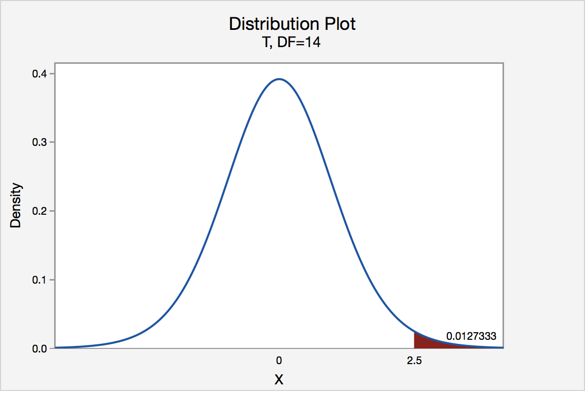
t-distrbution graph showing the right tail beyond a t value of 2.5

The P-value, 0.0127, tells us it is "unlikely" that we would observe such an extreme test statistic t* in the direction of H_A if the null hypothesis were true. Therefore, our initial assumption that the null hypothesis is true must be incorrect. That is, since the P-value, 0.0127, is less than $\alpha$ = 0.05, we reject the null hypothesis H₀ : μ = 3 in favor of the alternative hypothesis H_A : μ > 3.

Note that we would not reject H₀ : μ = 3 in favor of H_A : μ > 3 if we lowered our willingness to make a Type I error to $\alpha$ = 0.01 instead, as the P-value, 0.0127, is then greater than $\alpha$ = 0.01.

Left Tailed

In our example concerning the mean grade point average, suppose that our random sample of n = 15 students majoring in mathematics yields a test statistic t* instead of equaling -2.5. The P-value for conducting the left-tailed test H₀ : μ = 3 versus H_A : μ < 3 is the probability that we would observe a test statistic less than t* = -2.5 if the population mean μ really were 3. The P-value is therefore the area under a t_{n - 1} = t₁₄ curve and to the left of the test statistic t* = -2.5. It can be shown using statistical software that the P-value is 0.0127. The graph depicts this visually.

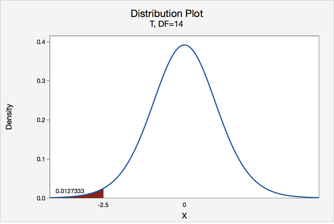
t distribution graph showing left tail below t value of -2.5

The P-value, 0.0127, tells us it is "unlikely" that we would observe such an extreme test statistic t* in the direction of H_Aif the null hypothesis were true. Therefore, our initial assumption that the null hypothesis is true must be incorrect. That is, since the P-value, 0.0127, is less than α = 0.05, we reject the null hypothesis H₀ : μ = 3 in favor of the alternative hypothesis H_A : μ < 3.

Note that we would not reject H₀ : μ = 3 in favor of H_A : μ < 3 if we lowered our willingness to make a Type I error to α = 0.01 instead, as the P-value, 0.0127, is then greater than $\alpha$ = 0.01.

Two-Tailed

In our example concerning the mean grade point average, suppose again that our random sample of n = 15 students majoring in mathematics yields a test statistic t* instead of equaling -2.5. The P-value for conducting the two-tailed test H₀ : μ = 3 versus H_A : μ ≠ 3 is the probability that we would observe a test statistic less than -2.5 or greater than 2.5 if the population mean μ really was 3. That is, the two-tailed test requires taking into account the possibility that the test statistic could fall into either tail (hence the name "two-tailed" test). The P-value is, therefore, the area under a t_{n - 1} = t₁₄ curve to the left of -2.5 and to the right of 2.5. It can be shown using statistical software that the P-value is 0.0127 + 0.0127, or 0.0254. The graph depicts this visually.

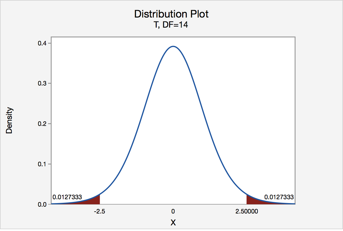
t-distribution graph of two tailed probability for t values of -2.5 and 2.5

Note that the P-value for a two-tailed test is always two times the P-value for either of the one-tailed tests. The P-value, 0.0254, tells us it is "unlikely" that we would observe such an extreme test statistic t* in the direction of H_Aif the null hypothesis were true. Therefore, our initial assumption that the null hypothesis is true must be incorrect. That is, since the P-value, 0.0254, is less than α = 0.05, we reject the null hypothesis H₀ : μ = 3 in favor of the alternative hypothesis H_A : μ ≠ 3.

Note that we would not reject H₀: μ = 3 in favor of H_A : μ ≠ 3 if we lowered our willingness to make a Type I error to α = 0.01 instead, as the P-value, 0.0254, is then greater than $\alpha$ = 0.01.

Now that we have reviewed the critical value and P-value approach procedures for each of the three possible hypotheses, let's look at three new examples — one of a right-tailed test, one of a left-tailed test, and one of a two-tailed test.

The good news is that, whenever possible, we will take advantage of the test statistics and P-values reported in statistical software, such as Minitab, to conduct our hypothesis tests in this course.

S.3.3 Hypothesis Testing Examples

Brinell Hardness Scores

An engineer measured the Brinell hardness of 25 pieces of ductile iron that were subcritically annealed. The resulting data were:

Brinell Hardness of 25 Pieces of Ductile Iron
170	167	174	179	179	187	179	183	179
156	163	156	187	156	167	156	174	170
183	179	174	179	170	159	187

The engineer hypothesized that the mean Brinell hardness of all such ductile iron pieces is greater than 170. Therefore, he was interested in testing the hypotheses:

H₀ : μ = 170
H_A: μ > 170

The engineer entered his data into Minitab and requested that the "one-sample t-test" be conducted for the above hypotheses. He obtained the following output:

Descriptive Statistics

N	Mean	StDev	SE Mean	95% Lower Bound
25	172.52	10.31	2.06	168.99

$\mu$: mean of Brinelli

Test

Null hypothesis H₀: $\mu$ = 170
Alternative hypothesis H₁: $\mu$ > 170

T-Value	P-Value
1.22	0.117

The output tells us that the average Brinell hardness of the n = 25 pieces of ductile iron was 172.52 with a standard deviation of 10.31. (The standard error of the mean "SE Mean", calculated by dividing the standard deviation 10.31 by the square root of n = 25, is 2.06). The test statistic t* is 1.22, and the P-value is 0.117.

If the engineer set his significance level α at 0.05 and used the critical value approach to conduct his hypothesis test, he would reject the null hypothesis if his test statistic t* were greater than 1.7109 (determined using statistical software or a t-table):

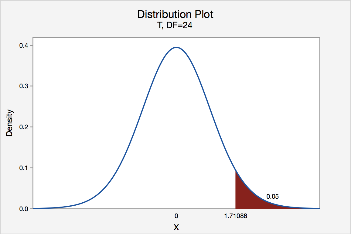
t distribution graph for df = 24 and a right tailed test of .05 significance level

Since the engineer's test statistic, t* = 1.22, is not greater than 1.7109, the engineer fails to reject the null hypothesis. That is, the test statistic does not fall in the "critical region." There is insufficient evidence, at the $\alpha$ = 0.05 level, to conclude that the mean Brinell hardness of all such ductile iron pieces is greater than 170.

If the engineer used the P-value approach to conduct his hypothesis test, he would determine the area under a t_{n - 1} = t₂₄ curve and to the right of the test statistic t* = 1.22:

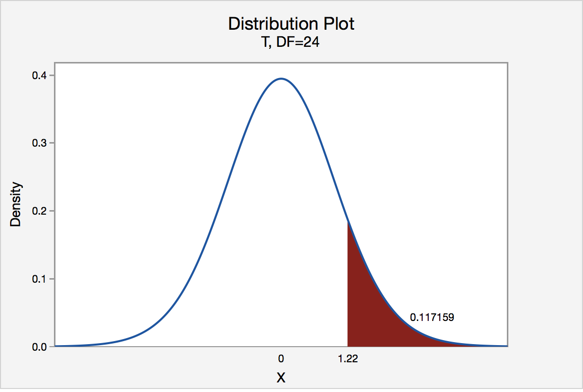
t distribution graph of right tailed test showing the p-value of 0117 for a t-value of 1.22

In the output above, Minitab reports that the P-value is 0.117. Since the P-value, 0.117, is greater than $\alpha$ = 0.05, the engineer fails to reject the null hypothesis. There is insufficient evidence, at the $\alpha$ = 0.05 level, to conclude that the mean Brinell hardness of all such ductile iron pieces is greater than 170.

Note that the engineer obtains the same scientific conclusion regardless of the approach used. This will always be the case.

Height of Sunflowers

A biologist was interested in determining whether sunflower seedlings treated with an extract from Vinca minor roots resulted in a lower average height of sunflower seedlings than the standard height of 15.7 cm. The biologist treated a random sample of n = 33 seedlings with the extract and subsequently obtained the following heights:

Heights of 33 Sunflower Seedlings
11.5	11.8	15.7	16.1	14.1	10.5	9.3	15.0	11.1
15.2	19.0	12.8	12.4	19.2	13.5	12.2	13.3
16.5	13.5	14.4	16.7	10.9	13.0	10.3	15.8
15.1	17.1	13.3	12.4	8.5	14.3	12.9	13.5

The biologist's hypotheses are:

H₀ : μ = 15.7
H_A: μ < 15.7

The biologist entered her data into Minitab and requested that the "one-sample t-test" be conducted for the above hypotheses. She obtained the following output:

Descriptive Statistics

N	Mean	StDev	SE Mean	95% Upper Bound
33	13.664	2.544	0.443	14.414

$\mu$: mean of Height

Test

Null hypothesis H₀: $\mu$ = 15.7
Alternative hypothesis H₁: $\mu$ < 15.7

T-Value	P-Value
-4.60	0.000

The output tells us that the average height of the n = 33 sunflower seedlings was 13.664 with a standard deviation of 2.544. (The standard error of the mean "SE Mean", calculated by dividing the standard deviation 13.664 by the square root of n = 33, is 0.443). The test statistic t* is -4.60, and the P-value, 0.000, is to three decimal places.

Minitab Note. Minitab will always report P-values to only 3 decimal places. If Minitab reports the P-value as 0.000, it really means that the P-value is 0.000....something. Throughout this course (and your future research!), when you see that Minitab reports the P-value as 0.000, you should report the P-value as being "< 0.001."

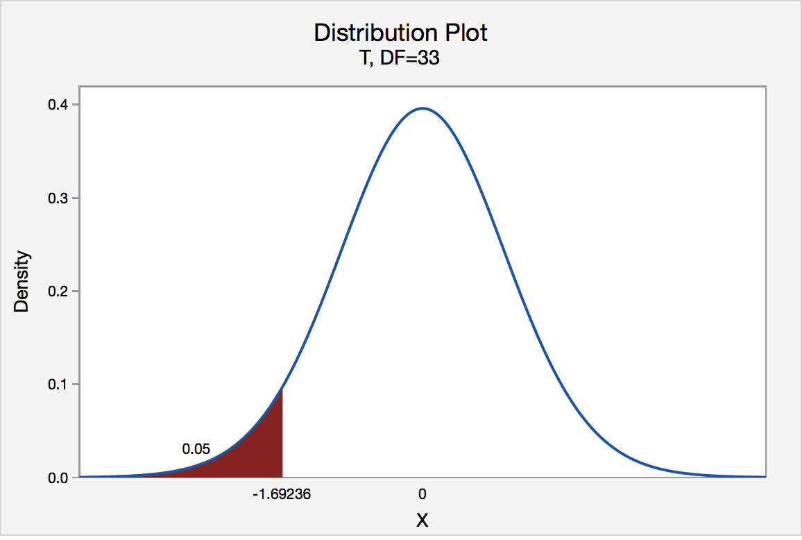
If the biologist set her significance level $\alpha$ at 0.05 and used the critical value approach to conduct her hypothesis test, she would reject the null hypothesis if her test statistic t* were less than -1.6939 (determined using statistical software or a t-table):s-3-3

Since the biologist's test statistic, t* = -4.60, is less than -1.6939, the biologist rejects the null hypothesis. That is, the test statistic falls in the "critical region." There is sufficient evidence, at the α = 0.05 level, to conclude that the mean height of all such sunflower seedlings is less than 15.7 cm.

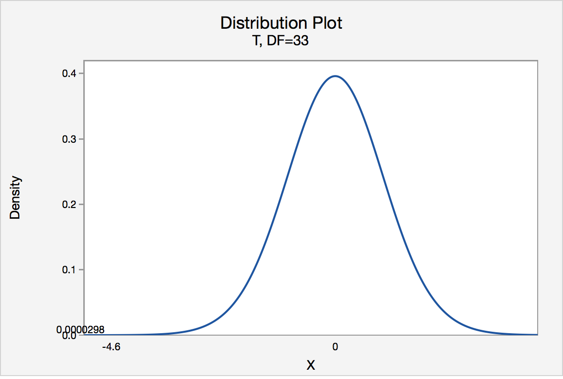
If the biologist used the P-value approach to conduct her hypothesis test, she would determine the area under a t_{n - 1} = t₃₂ curve and to the left of the test statistic t* = -4.60:

t-distribution for left tailed test with significance level of 0.05 shown in left tail

In the output above, Minitab reports that the P-value is 0.000, which we take to mean < 0.001. Since the P-value is less than 0.001, it is clearly less than $\alpha$ = 0.05, and the biologist rejects the null hypothesis. There is sufficient evidence, at the $\alpha$ = 0.05 level, to conclude that the mean height of all such sunflower seedlings is less than 15.7 cm.

t-distribution graph for left tailed test with a t-value of -4.60 and left tail area of 0.000

Note again that the biologist obtains the same scientific conclusion regardless of the approach used. This will always be the case.

Gum Thickness

A manufacturer claims that the thickness of the spearmint gum it produces is 7.5 one-hundredths of an inch. A quality control specialist regularly checks this claim. On one production run, he took a random sample of n = 10 pieces of gum and measured their thickness. He obtained:

Thicknesses of 10 Pieces of Gum
7.65	7.60	7.65	7.70	7.55
7.55	7.40	7.40	7.50	7.50

The quality control specialist's hypotheses are:

H₀ : μ = 7.5
H_A: μ ≠ 7.5

The quality control specialist entered his data into Minitab and requested that the "one-sample t-test" be conducted for the above hypotheses. He obtained the following output:

Descriptive Statistics

N	Mean	StDev	SE Mean	95% CI for $\mu$
10	7.550	0.1027	0.0325	(7.4765, 7.6235)

$\mu$: mean of Thickness

Test

Null hypothesis H₀: $\mu$ = 7.5
Alternative hypothesis H₁: $\mu \ne$ 7.5

T-Value	P-Value
1.54	0.158

The output tells us that the average thickness of the n = 10 pieces of gums was 7.55 one-hundredths of an inch with a standard deviation of 0.1027. (The standard error of the mean "SE Mean", calculated by dividing the standard deviation 0.1027 by the square root of n = 10, is 0.0325). The test statistic t* is 1.54, and the P-value is 0.158.

If the quality control specialist sets his significance level $\alpha$ at 0.05 and used the critical value approach to conduct his hypothesis test, he would reject the null hypothesis if his test statistic t* were less than -2.2616 or greater than 2.2616 (determined using statistical software or a t-table):

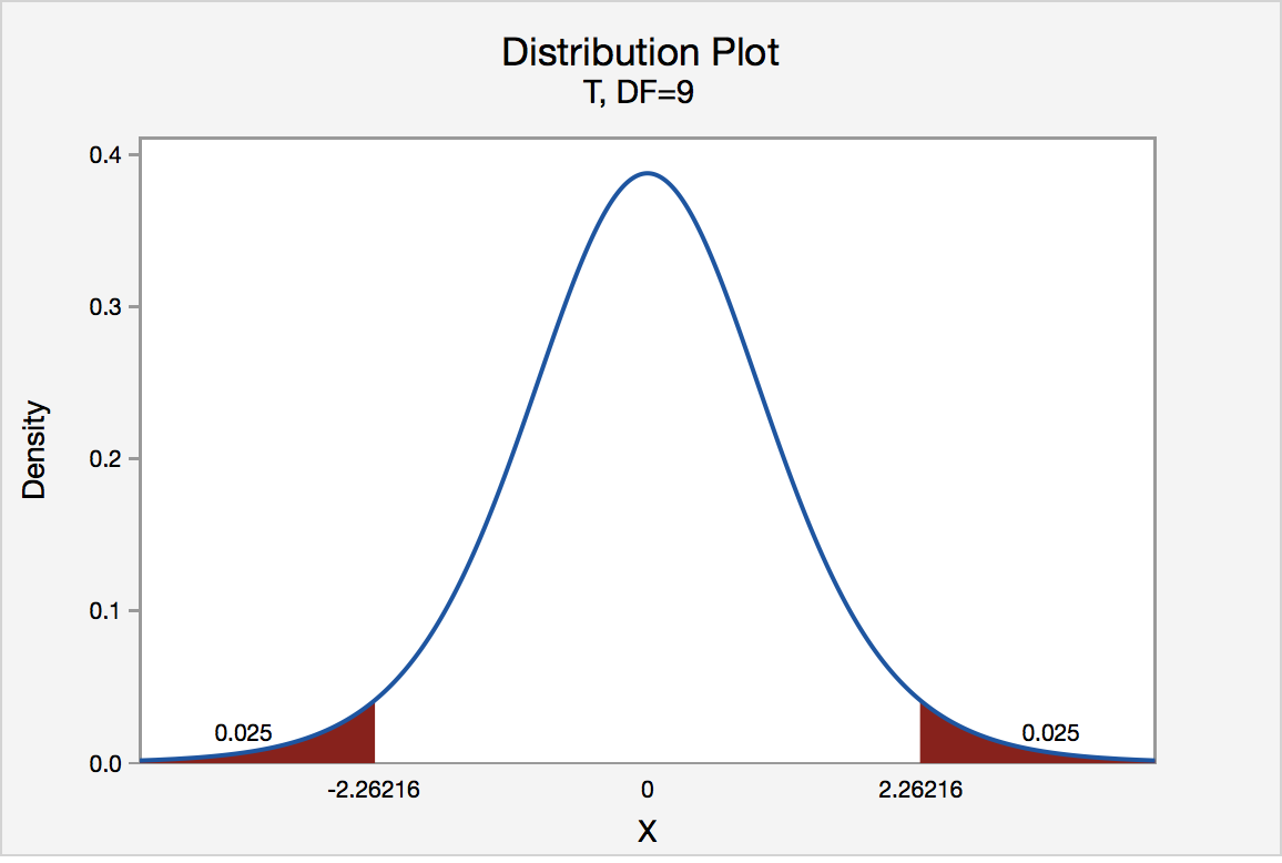
t-distribution graph of two tails with a significance level of .05 and t values of -2.2616 and 2.2616

Since the quality control specialist's test statistic, t* = 1.54, is not less than -2.2616 nor greater than 2.2616, the quality control specialist fails to reject the null hypothesis. That is, the test statistic does not fall in the "critical region." There is insufficient evidence, at the $\alpha$ = 0.05 level, to conclude that the mean thickness of all of the manufacturer's spearmint gum differs from 7.5 one-hundredths of an inch.

If the quality control specialist used the P-value approach to conduct his hypothesis test, he would determine the area under a t_{n - 1} = t₉ curve, to the right of 1.54 and to the left of -1.54:

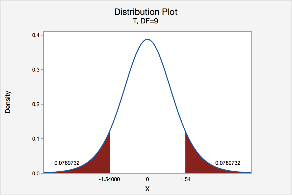
t-distribution graph for a two tailed test with t values of -1.54 and 1.54, the corresponding p-values are 0.0789732 on both tails

In the output above, Minitab reports that the P-value is 0.158. Since the P-value, 0.158, is greater than $\alpha$ = 0.05, the quality control specialist fails to reject the null hypothesis. There is insufficient evidence, at the $\alpha$ = 0.05 level, to conclude that the mean thickness of all pieces of spearmint gum differs from 7.5 one-hundredths of an inch.

Note that the quality control specialist obtains the same scientific conclusion regardless of the approach used. This will always be the case.

In closing

In our review of hypothesis tests, we have focused on just one particular hypothesis test, namely that concerning the population mean $\mu$. The important thing to recognize is that the topics discussed here — the general idea of hypothesis tests, errors in hypothesis testing, the critical value approach, and the P-value approach — generally extend to all of the hypothesis tests you will encounter.

^[1]	Link
↥	Has Tooltip/Popover
	Toggleable Visibility

Brinell Hardness of 25 Pieces of Ductile Iron
170	167	174	179	179	187	179	183	179
156	163	156	187	156	167	156	174	170
183	179	174	179	170	159	187

Brinell Hardness of 25 Pieces of Ductile Iron
170	167	174	179	179	187	179	183	179
156	163	156	187	156	167	156	174	170
183	179	174	179	170	159	187

Brinell Hardness of 25 Pieces of Ductile Iron
170	167	174	179	179	187	179	183	179
156	163	156	187	156	167	156	174	170
183	179	174	179	170	159	187