Another application of the Kolmogorov-Smirnov statistic is in forming a confidence band for an unknown distribution function \(F(x)\). To form a confidence band for \(F(x)\), we basically need to find a confidence interval for each value of x. The following theorem gives us the recipe for doing just that.
A \(100(1−\alpha)\%\) confidence band for the unknown distribution function \(F(x)\) is given by \(F_L(x)\) and \(F_U(x)\) where d is selected so that \(P(D_n ≥ d) = \alpha\) and:
and:
Proof
We select d so that:
\[P(D_n \ge d)=\alpha\]
Therefore, using the definition of \(D_n\), and the probability rule of complementary events, we get:
\[P(sup_x|F_n(x) -F(x)| \le d) =1-\alpha\]
Now, if the largest of the absolute values of \(F_n (x) - F(x)\) is less than or equal to d, then all of the absolute values of \(F_n (x) - F(x)\) must be less than or equal to d. That is:
\[P\left(|F_n(x) -F(x)| \le d \text{ for all } x\right) =1-\alpha\]
Rewriting the quantity inside the parentheses without the absolute value, we get:
\[P\left(-d \le F_n(x) -F(x) \le d \text{ for all } x\right) =1-\alpha\]
And, subtracting \(F_n (x)\) from each part of the resulting inequality, we get:
\[P\left(- F_n(x)-d \le -F(x) \le -F_n(x)+d \text{ for all } x\right) =1-\alpha\]
Now, when we divide through by −1, we have to switch the order of the inequality, getting:
\[P\left(F_n(x)-d \le F(x) \le F_n(x)+d \text{ for all } x\right) =1-\alpha\]
We could stop there and claim that:
\[F_n(x)-d \le F(x) \le F_n(x)+d \text{ for all } x\]
is a \(100(1−\alpha)\%\) confidence band for the unknown distribution function \(F(x)\). There's only one problem with that. It is possible that the lower limit is less than 0 and it is possible that the upper limit is greater than 1. That's not a good thing given that a distribution function must be sandwiched between 0 and 1, inclusive. We take care of that by rewriting the lower limit to prevent it from being negative:
and by rewriting the upper limit to prevent it from being greater than 1:
As was to be proved!
Let's try it out an example.
Example 22-4 Section

Each person in a random sample of n = 10 employees was asked about X, the daily time wasted at work doing non-work activities, such as surfing the internet and emailing friends. The resulting data, in minutes, are as follows:
108 112 117 130 111 131 113 113 105 128
Use the data to find a 95% confidence band for the unknown cumulative distribution function \(F(x)\).
Answer
As before, we start by ordering the x values. The formulas for the lower and upper confidence limits tell us that we need to know d and \(F_n (x)\) for each of the 10 data points. Because the \(\alpha\)-level is 0.05 and the sample size n is 10, the table of Kolmogorv-Smirnov Acceptance Limits in the back of our text book, that is, Table VIII, tells us that \(d = 0.41\). We already calculated \(F_n (x)\) in the previous example.
Now, in calculating the lower limit, \(F_L(x) = F_n (x) − d = F_n (x)−0.41\), we see that the lower limit would be negative for the first four data points:
0.1−0.41 = −0.31 and 0.2−0.41 = −0.21 and 0.3−0.41 = −0.11 and 0.4−0.41 = −0.01
Therefore, we assign the first four data points a lower limit of 0, and then just calculate the remaining lower limit values. Similarly, in calculating the upper limit, \(F_U (x) = F_n (x) + d = F_n (x) + 0.41\), we see that the upper limit would be greater than 1 for the last six data points:
0.6+0.41 = 1.01 and 0.7+0.41 = 1.11 and 0.8+0.41 = 1.21 and 0.9+0.41 = 1.31 and 1.0+0.41 = 1.41
Therefore, we assign the last six data points an upper limit of 1, and then just calculate the remaining upper limit values. To summarize,
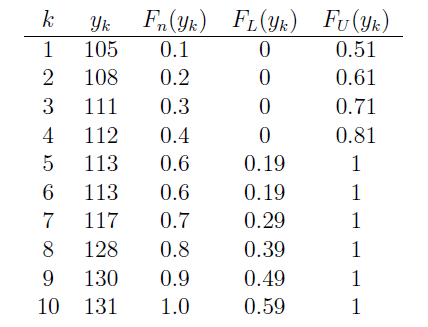
The last two columns together give us the 95% confidence band for the unknown cumulative distribution function \(F(x)\).