Printer-friendly version

Often we have specific hypotheses that we want to test such as "Gene X is over-expressed in tumor samples" or "People with colon cancer are more likely to have SNP Y".

Classical Statistical Tests

In classical (frequentist) statistics, we do not try to obtain the probability that our hypothesis is true.  Instead, we set up a null hypothesis that would be false if our hypothesis is true.  We then try to determine if the observed data are surprising if the null hypothesis is true. What do we mean by surprising?  If a sample at least as unusual as the observed could have happened by chance it's not surprising. If it happens by chance only with low probability, then it is surprising.

Classical statistical testing is therefore based on a thought experiment: First, we set up a null hypothesis and compute the sampling distribution of our summary (call the test statistic) when the null hypothesis is true.  Notice that we can do this without observing any data, because it is based on a thought experiment.  Then we take a sample and compute the test statistic.  Finally, we compute the probability that a test statistic at least as extreme as the observed value would be if the statistic were selected at random from the sampling distribution we obtain assuming the null hypothesis is true.  This probability is called the p-value of the test.  If the p-value is small we reject the null hypothesis and state that there is evidence against the null.  

To do classical hypothesis testing, we set up two hypotheses. 1) The null hypothesis, which we hope to find evidence against. 2) The alternative hypothesis, which  we provide as the alternative source of the data if there is evidence against the null.  Note, however, that all probability statements are based on the null hypothesis; evidence against the null does not indicate than any particular alternative is more likely.

For example, if we're looking at gene expression in tumor versus normal tissue our hypotheses would be:

H₀: the gene does not differentially express (on average)
H_A: the gene does differentially expresses (on average)

If we are looking at drug treatments, the null hypothesis is that the mean response on the drug and on the placebo is the same. The alternative hypothesis is that there is a difference.

The tests that we will start out with required that the data are independent, and usually that they have the same spread or variability under all the conditions of interest. Taking logarithms helps equalize variance for most gene expression data.  Boxplots can be used to visualize the data and its spread to see how well this assumption holds.

Independence of the data cannot be determined by looking at a table of numbers. Independence is something that comes from the study design.  Dependence is usually due to biology, environment or both.  For example, samples taken from the same subject are dependent due to both genetics and shared environment.  Samples taken from clones reared separately are dependent due to genetics.  Samples taken from unrelated subjects reared together are dependent due to environment.

What is a p-value?

Notice that the p-value is not the probability that either of the two hypotheses is true.  The p-value is the probability that a sample selected at random produces a value of the test statistic at least as extreme as the observed value when H₀ is true.  We can think of the p-value as measure of how surprising our result is if the null hypothesis is true.  If the p-value  is small, we reject our null hypothesis H₀.

" p is small" is often interpreted as p is < 0.05 (significant) which means that we would see something that was surprisingly 5% of the time  if the null hypothesis is true.   p-value is < 0.01  would be even more surprising if the null hypothesis is true, and is often denoted as highly significant. However,  a typical way to handle high throughput data is to do a test for each feature. So, if we're measuring gene expression for a whole genome and measure 50,000 features, or are doing a GWAS study where we might be doing 2 million tests, events that happen by chance 5% of even 1% of the time are expected.    For example, suppose that we measure 50,000 features in two sets of samples from the same population.  We know that at the population level there is no differential expression, but 50,000*0.05=2500 test statistics will be statistically significant at p<0.05 and even at p<0.01 we will have 500 significant tests.  These are all "false discoveries".  

To handle this we will talk about multiple testing later along with false discovery rates and false non-discovery rates, to try to understand this issue and how to deal with it when doing a high throughput study.  A simulation study later will help us understand how this works.

Example: Colon Cancer Data, cont'd

Does  HSA.4689 express differently in tumor cells compared to normal cells?

40 samples are from tumor biopsies - 't'
22 samples are from normal biopsies - 'n'

2000 (of 6500) probes were selected for analysis

This graph below shows the observed distribution of log2(expression) in the normal and tumor tissue.

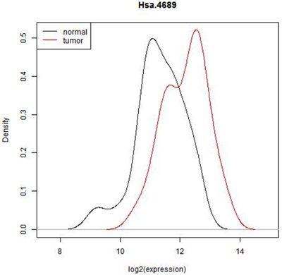
In some situations it is pretty clear that there is a difference in expression -  all of the normal tissue samples have lower expression of this feature and all of the tumor samples have a higher expression or vice versa. In that case, we really wouldn't need to do a statistical test. ( In fact, we might have to because the reviewer of our paper might insist on it but the result would be obvious!) However here is there considerable overlap. Expression seems to be shifted up in tumor, but there are only 22 normal and 40 tumor biopsies- perhaps expression is really the same and we just happened by chance to pick a sample with a few smaller values in the normal tissue and a few higher values in the tumor tissue. In fact, we can see that if we just select one random value from the normal samples and one from the tumor samples either one could be higher.  Even if we conclude after testing that mean expression of this gene is higher in tumor cells, we will not be able to avoid the fact that most expression values are similar for both cell types.

Notice that what is plotted here is log2(expression).  Gene expression values are often skewed with many low values and a few high ones.  There are statistical testing methods that can deal with skewed data, but they are not very flexible.  log2(expression) is closer to a Bell-shaped distribution for which we can use some very powerful and flexible methods.  Expression data is almost always analyzed on the logarithmic scale.

Additionally, one thing that the histogram does not show is the pairing of normal and tumor samples. When we looked at the scatterplot matrix of all the samples together, we saw the two samples from the same patient were much more similar two each other than to normal samples from different patients or two tumor samples from two patients. This pairing is hidden in this histogram.

Although it might be more interesting to ask whether, for this gene, the distribution of gene expression differs between normal and tumor tissue, answering this very general question requires a lot of data.  It might also be too general for our needs.  Typically, we formulate the null hypothesis in terms of a small set of parameters of the populations, such as the means.

The inferential question we are asking is whether there is a difference in the two population means. We can determine directly from the data whether there is a difference in the sample means, but this is only one possible outcome from all of the possible samples that could be taken of normal and tumor colon tissue.  In short, we need to know the sampling distribution of the difference in sample means.  

Recall that we set up a null hypothesis that we want to show as false. If we're looking for differential expression,the null hypothesis is that there is no differential expression, that is the mean expression levels are equal. Usually we don't know to advance whether our genes are over or under-expressed, so our alternative hypothesis is just that the means are not equal.

We set up a null and alternative hypothesis in the following manner:

Let X be the log2(expression) in the normal samples with mean \(\mu_X\).
Let Y be the log2(expression) in the tumor samples with mean \(\mu_Y\).

\(H_0: \mu_X=\mu_Y\) or \(H_0: \mu_X-\mu_Y=0\)
\(H_A: \mu_X\neq\mu_Y\) or \(H_A: \mu_X-\mu_Y\neq0\)

The null hypothesis is that the two means of the same and the alternative is that they are different. Often convenient express the null and alternative hypotheses in terms of the difference, i.e. the difference in the means is zero or not zero. We then set up a experiment and our statistical tests so that we can compute the probability of observing a value of the test statistic as extreme or more extreme than the observed value if the null hypothesis is true.

We estimate \(\mu_X\) by \(\bar{X}\) and the variance of X by \(S_X^2\).
We estimate \(\mu_Y\) by \(\bar{Y}\) and the variance of Y by \(S_Y^2\).

If the null hypothesis is true, we expect \(\bar{X}-\bar{Y}\) to be close to zero.  The question is: how far from zero does the difference need to be for us to reject the null?   Here is where we use the thought experiment. The mean of the sampling distribution of  \(\bar{X}-\bar{Y}\)  is \(\mu_X-\mu_Y\).   We would reject the null hypothesis if the probability of observing a value in the sampling distribution at least as extreme as the observed value is small.

The problem is that we have only one observation - how can we obtain the sampling distribution (or an estimate of the sampling distribution).  This is where the thought experiment comes in.  We are going to consider both an intuitive method (permutation tests) and a method based on statistical theory (t-tests).  The great statistician and genomicist R.A. Fisher thought of the t-test as an approximation to the permutation test, but these days we usually think of permutation tests as suitable when we do not want to make assumptions about the shape of the underlying population (nonparametric) and t-tests when we assume that the underlying population is not too far from Normal (parametric).

Permutation Test

The idea in permutation testing is that if there is no difference in means then the gene expression observed in the  sample is equally likely to have come from the normal or tumor tissue.  We cannot take any new samples, but we could re-assign the values at random to the normal or tumor tissues, by taking the 66 sample labels and just randomly changing their order.  Actually, we should not do this due to the pairs of samples that came from the same patient, so lets limit ourselves to one sample per patient - the 22 normal samples and the 18 tumor samples that came from the patients who provided only tumor samples.  

So, now there are 40 samples, of which 22 are normal and 18 are tumor.  In the permutation test, we simply mix up the samples at random (or equivalently, mix up the labels.)  There are a lot of different ways to do this (11,3380,261,800), and computing the difference in means each way gives us an empirical estimate of the null distribution called the permutation distribution.  Of course, we will not compute all of the values - a few thousand at most to approximate the null distribution.  Suppose that take our original 40 samples and assign 22 at random to the "normal" label and the other 18 to tumor.  We then compute the difference in sample means.  We do this independently 10,000 times.  We then go back to our original value, which is -0.914.  We look at the permutation distribution and see how many values are greater than or equal to 0.914 OR less than or equal to -0.914  That tells us how extreme the observed value is if it actually comes from the null distribution distribution.  (Remember, this distribution assumes that there is no difference in expression between the normal and tumor samples.)  If the observed value is in the typical region, we accept the null hypothesis.  If not, we reject the null.

We do this in the demo below.  (It will be much clearer if you view it in full screen mode.)  I have also uploaded Permutation.Rmd which you can use if you want to try this yourself.  Remember that the permutations are created at random, so you will not get the exact same answer that I did.

But there is a big problem with what we have done - we have not used all the samples.  It is easy to use this method when all the samples are independent (and this is what was demonstrated).  It is also easy to use this method when all the samples are paired (for each patient flip a coin and swap labels when the coin is a head).  But it is difficult to do permutation tests when we have a mix of paired and unpaired samples - especially when all the unpaired samples come from the same condition (tumor in this case).

We will consider t-tests in the next section.  However, we will not consider tests using all the samples until later in the semester when we cover linear models.