3.4 - Steps in Designing a Study
Here is a classical view of how a study proceeds.
- Determine the objective of your study.
- Determine the experiment conditions (treatments).
- Determine the measurement platform
- Determine the biological sampling design.
- Determine the biological and technical replicates.
- Determine the sequencing depth
- Determine the tissue pool
- Determine the measurement
- Do the study
What's missing here is the study sequence. You do a study, analyze the data and generate hypotheses which leads to the next experiment. We talk about the experiment as if it is done in isolation, but this is almost never the case. We hope that any flaws in our earlier findings will be exposed by the experiments that follow and that any correct findings will be strengthened. We often hope that the later studies will refine our results - e.g. after finding that a gene over-expresses in tumor tissue, we might find that this is limited to a region of the tissue or a time-point in tumor development. Most statistical analysis is done on a "one experiment at a time" basis but scientific advances require a series of experiments. A particular experimental design might seem optimal for a single experiment in the series, but its efficacy has to be judged in the context of its value as part of the entire series.
Lets look at some of the steps in more detail.
1. Determine the Objective of Your Study
The level of replication should match the objectives. For differential analysis, we compare the mean difference between treatments to the variability among the replicates. For clustering we averaged among replicates of the correct level. In either case, we need to decide the appropriate level of replication. For example, for a study of tumor development in mice we might decide to use one tumor per mouse in several mice. However if the mice typically develop several tumors, we might prefer to sample 2 tumors per mouse to determine if within mouse variability is smaller than between mouse variability. If the tumor appear to be quite spatially heterogeneous, we might consider sampling several spatial locations in the tumor.
We also need to think ahead about the type of analysis that will be done. For example, if we're doing a differential analysis, we will do a t-test or something like a t-test. We will need the means and the variances. If we're doing a clustering analysis, i.e. clustering tumors based on their gene expression we would usually average the tumors of the same type before clustering.
As discussed earlier, you need to balance biological versus technical replicates. We usually don't need to need technical replicates unless you're interested in knowing what the measurement error is. However, when biological replication is expensive compared to technical replication (for example, when the specimens are very rare - e.g. mammoth tissue - or difficult to sample - e.g. growth tip of a root hair) then technical replication can help you by reducing measurement error.
2. Determine the Experiment Conditions (treatments) Under Study.
You need to determine the factors in your experiment, their levels and which combinations you will use as treatments.
Typically our studies are comparative, with 2 or more treatments. Factor levels should be selected that you expect to have biologically significant differences. For example, if you are studying exposure to a toxin under experimental control, it is useful to have some a priori information about the exposures that will produce effects ranging from minimal to highly toxic. If this type of information is not available, it is useful to run a small pilot experiment to determine the appropriate doses.
If there is some sort of stimulus, it is good to have a control condition. Control conditions are not always clearly defined - for example, if a drug is injected in mice, should the control be "no injection", "injection of saline solution" or some other preparation, such as "injection with drug solvent"? When using organisms with some type of mutation, the wild-type from the same genetic background is usually used as the control. Ethical standards also need to be considered - in animal and especially human studies, placebos are not always ethically be used as controls. In these cases, the "control" should be the gold standard treatment, against with a newer treatment can be compared.
Many experiments have a single factor with 2 or more levels. In this case, each level is a treatment, and many levels may be used. When there are 2 or more factors, the usual design is the factorial (also called crossed) design which uses all level combinations as treatments..
Example of factorial design with two Genotypes, two Tissue types and 3 Times
For a study with 2 genotypes (G and g), 2 tissue samples (T and t), at three times (a, b and c). The treatments would be:
| GTa | GTb | GTc |
| Gta | Gtb | Gtc |
| gTa | gTb | gTc |
| gta | gtb | gtc |
If you do the entire factorial set up, you will have all 2x2x3=12 combinations as part of your experiment. Since replication is required, this experiment needs at least of 24 observations to replicate everything.
You can see that designs with multiple factors at multiple levels can be very expensive due to the number of treatments. More compact designs which do not use all combinations but which are almost as informative can be constructed, but are seldom used in biology (although they are heavily used in industry). If you need to vary more than 3 factors in an experiment, seek statistical assistance.
Statisticians will say that the design is said to be balanced if there are equal numbers of replicants all levels for all conditions. This turns out to be useful in terms of a robustness against assumptions about the distributions of the populations. Statistically, problems such as nonnormality and differences in variance don't matter as much when we have equal sample sizes. However, we are not always constrained to have equal sample sizes: some factor levels may be difficult to sample or expensive to apply (for example, rare genotypes or expensive drugs); equipment fails, mice die of causes not related to the experiment, nucleotide samples degrade or are lost. Unbalanced experiments can be analyzed statistically. However, the interpretation of badly unbalanced experiments may be difficult and may require additional statistical input.
Time is often a factor in experiments that may involve biological processes such as growth or tissue damage. In biology, experiments over time are often called "time-course" experiments. Statisticians may refer to these differently. When independent biological entities are sampled at the different times, (say groups of plants that are pulled up at weeks 1 and 3) the statistician just considers this a factor like any other, and assign the samples at random to the sampling time. However, when a biological entity is sampled repeatedly over time, this is called a longitudinal or repeated measures design. When a time course design has repeated measurements on the same individual, this needs to be taken into account in the statistical analysis. We usually assume that there is correlation among the samples from the same individual, which reduces their variability compared to samples taken from different individuals. Use of repeated measures can improve power for detecting differences by reducing the variability of the comparisons (thereby improving the false negative rate), but ignoring the correlation when doing the analysis leads to a larger false positive rate. Biologists need to distinguish between the two types of time course studies.
In time course experiments, the times do not need to be equally spaced. Just as in "dosing" studies, it is important to have some a priori idea of what times will be interesting. As well, it is important when possible to start with samples that are in some sense synchronized, so that "time 0" means the same thing to every sample. However, even when the samples are synchronized at the start of the study, they may be out of synchrony as time goes on, which will lead to greater variability at later time points.
Finally, in multifactor studies we may need to redefine the levels for some factors. For example, suppose we are growing larvae at different temperatures - we may need to measure time by growth stage rather than elapsed time to make meaningful comparisons. Suppose we are looking at exposures to a toxin and we have susceptible and resistant genotypes: should dose of toxin be the level, or is it more meaningful to use some measure of damage? Choice of levels should be determined by the biological hypotheses under study.
3. Determine the Measurement Platform
At some point, usually while you are figuring out budgets, you will need to figure out what the measurement platform should be. Over time, more platforms are becoming available and measurement costs are rapidly decreasing. However, data storage and analysis costs are not declining. Choice of platform is a complex decision.
The platform and reagent manufactures and the technical staff at the microarray or sequencing center are valuable sources of information about the pros and cons of the measurement platforms. At Penn State, the staff in the Genomics Core in the Huck Institutes of Life Sciences are both knowledgeable and helpful. That being said, much innovative work is being done in research labs developing novel methodology with these technologies.
Cost and accuracy are major considerations in selecting technologies and experimental designs within technologies. There are several components to cost - sample preparation, running the samples, and handling the resulting data. There are also less tangible costs which come from nost getting all the required information from the experiment.
You need to consider the cost of 'doing it right'versus the cost of:
- Repeating the entire experiment,
- validating all findings on another platform, or
- losing of publication, grant opportunity are precedence.
Often what is cheap on the surface is not cheap in the end. It is worth putting in the time to figure out the best experiment, the best platform, and so on before you do the experiment. Even if it turns out to be inexpensive to run the experiment, if you can't publish it you might as well not have done it.
In this course we are going to discuss the two currently most popular platforms, microarrays and short read high throughput sequencing. Single molecule sequencing is now also available and is relatively high throughput - humdreds of thousands of reads. However, millions of reads (sequences) are required to do statistical analyses such as differential expression analysis or genotyping. In any case, as long as the data are counts of molecules or fragments, the analysis should be quite similar to the analysis of short read data.
Microarrays
Microarray's for model species are very reliable now. Gene expression microarrays can be fairly readily designed for un-sequenced species using a new sequencing technologies. They are very good for comparative analysis but you can't find what is not on the array. You can get differential hybridization for reasons that are not directly due to gene expression. For instance, sequence variation, splice variation and other factors create differential hybridization.
Microarrays are being phased out for experimental work, but are cost-effective for many situations. Data management and data analysis costs are very minimal. Since probe development and printing are fairly inexpensive, microarrays can also be used for non-model species.
High Throughput Short-read Sequencing
High throughput short-read sequencing produces more information than microarrays. It seems to have a higher dynamic range, i.e. you can get the low-end and high-end information more accurately. It can be applied to any biological entity, including mixtures of organisms such as gut microflora. High throughput sequencing does not require knowing what you are looking for and is not affected by genetic variation (except in large insertions or deletions).The costs have come down dramatically in the past couple of years, due to ultra-high throughput and multiplexing (the ability to label multiple samples and sequence them simultaneously).
Data management is the biggest challenge. The dataset are huge - several gigabytes, so storing and moving the raw data is difficult. The sequences are identified by mapping to a reference genome or transcriptome. If there is no reference, then one must be created, which has its own unique challenges. For some studies, such as cancer transcriptomes, sequence variability may be high, so that considerable expertise and computing must be applied before the data are in a format suitable for statistical analysis.
High throughput sequencing is currently the platform of choice for most research studies. There are many design considerations after deciding to use short-read sequencing. Some of these are discussed in [1].
4. Determine the Biological Sampling Design
The sampling design consists of several components: determining how the samples will be collected, determining if blocking is appropriate and determining the number of types of replicates.
A block is a set of samples that in the absence of treatment effects have a natural clustering. Usually, the clustering means that there is less variability within blocks than between blocks. For example, in our colon cancer example, a person would be a block with the potential for taking 2 samples per person. However, there are lots of reasons why you need blocks. Some of these reasons have to do with having to tissue samples from the same individual. Another reason might be the set up of the experiment, i.e., the mice that are in the mouse house at the same time should have all the same environmental conditions and so they are more similar than mice housed at different times. Plants grown in the same field may be more similar than plants grown in different fields. Blocks may also be induced in an experiment due to technical issues induced by taking or processing samples in different labs, at different times or by different personnel.
It important to have a strong protocol for sample collection so that biases and extra variability are not introduced by, for example, different technicians handling the samples in slightly different ways, or collecting samples under different environmental conditions. Reducing variability by use of a strong protocol induces internal validity of the results - if the samples are collected and handled identically, then observed treatment differences should actually be due to the treatment. However, having too little variability in the samples can reduce external validity - the experimental results cannot be replicated at another time or in another lab because the new samples differ in some way that had been controlled by the protocol.
Balance between internal and external validity can be achieved by blocking. Samples in the same block should be very similar in the absence of treatment effects, while different blocks should reflect the variability of the population. For example, if the environmental conditions in the greenhouse are important for gene expression in leaf, samples can be collected over several days, with enough samples in a single day to perform an entire replicate of the experiment. This way, slight changes in humidity, temperature, lighting and other environmental factors will be sampled over the days, while kept very uniform at each sampling time. It might be even better if the plants can be grown in several batches and and a complete replicate of the experiment done on each batch, which would reflect variability in the growth conditions etc.
A common mistake is to confound a blocking factor with a treatment. For example, it might be more convenient to house one genotype at each lab. But if you want to compare genotypes, you will not be able to determine if the observed differences are due to genotype or due to lab differences.
In some situations, it is not possible to replicate an entire experiment in a block because the number of treatments is greater than the number of samples in the block. For example, in twin studies we have only 2 samples (the sibs) in each block. Another example is two sample microarrays, where we induce blocking by hybridizing two samples to the microarray probes. When the entire experiment cannot be done in a single block, special designs called incomplete block designs can be used to provide some of the variance reduction due to blocks while maintaining the balance of the experiment. Complete block designs and balanced incomplete block designs are very amenable to statistical analysis.
Regardless of whether you are using complete or incomplete blocks, if the randomization has been done within block, then block needs to be recorded. Blocking induces a type of correlation (the intraclass correlation) similar to the correlation in repeated measures designs. If it is not accounted for in the statistical analysis the false positive and false negative rates will be increased.
A note on jargon: Many biologists consider one replicate of the entire experiment to be an experiment and might state that they did 3 experiments. A statistician will call this three replicates or 3 blocks.
5. Determine the Number of Biological and Technical Replicates
Biological replication is used for statistical inference. The more biological replicates that you have, the higher your power. And because whenever you take a measurement, part of this measurement is measurement error, if you have enough biological replicates there is not any reason to take technical replicates unless you really want to know what the size of the measurement error is.
What is the right sample size? I used to say that it is always more than anyone can afford, but with the decreased cost of measurement, some large medical studies in humans have quite large sample sizes. However, in the scientific setting, we generally have to balance the cost of the current experiment with the cost of doing the follow-up experiments that might validate or refine our results. For this reason, we often set a sample size in advance and then try to estimate the power of the experiment to detect differences of various sizes.
At minimum you should have three biological replicates for treatment. That being said, dozens and dozens of experiments have only two replicates. These experiments have very high false discovery and false non-discovery rates. However, they can be useful to provide some rough measures of biological processes that can then be used as pilot experiments to to guide sample size estimation and experimental design for experiments with better replication.
Technical replication is essential when part of the experimental objective is to measure the measurement error. When the objectives are purely biological, technical replication is not as effective as biological replication. However, in some circumstances, technical replicates may be much less expensive - for example if the specimens are rare or the treatments are difficult to apply. In those cases, technical replication can be used to reduce the measurement error by averaging the replicates. Typically when answering biological questions, we want to compare the treatment effects to the natural biological variability of our samples. For this reason, we need to sample (and estimate) the full biological variability. Hence measurement error will only be one component of the sample variability and the variance reduction due to averaging technical replicates quickly declines in importance.
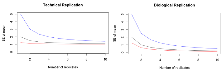
In the left figure, the black line shows the effects of technical replication on the SE of the mean when the biological variation and measurement variation are the same. The red line shows the effects of technical replication when the biological variation is 4 times larger than the error variation and the blue line shows the effects when the biological variation is 4 times smaller. Even with very large error variation, the effect of technical replication quickly asymptotes at the magnitude of the biological variation. In the right figure, the black line shows the effects of biological replication on the SE of the mean when the biological variation and measurement variation are the same. The red line shows the effects of biological replication when the biological variation is 4 times larger than the error variation and the blue line shows the effects when the biological variation is 4 times smaller. The curves asymptote at zero.
It is important to keep track of the blocks, biological replicates and technical replicates when recording sample information, as these features of the experiment are used for estimating variability. One of the sources of irreproducible statistical analyses is that the sample information is lost.
In sequencing studies, another important determinant of measurement error is the amount of sequencing done - i.e. the number of fragments sequenced per sample or sequencing depth. Increasing the sequencing depth, (getting more reads per sample), increases the power quite similarly to technical replication. As with technical replication, increasing the read depth reduces the measurement error (relative to the treatment effects) but just like technical replication, there is a non-zero asymptote for the total error. Sequencing depth must be traded off for additional biological replication.
The question still remains, how big should the sample be?
Appropriate sample sizes can be determined from a power analysis which requires an estimate of total variation and the sizes of the effects you hope to detect. You also need to specify the p-value at which you will reject the null hypothesis, and the desired power. For simple cases such as the t-test, R and other statistical software can provide an estimate.
In a high throughput experiment, each feature can have a different variance. Even if we agree that 2-fold difference is an appropriate target for effect sizes that should be detectable with high probability, the difference in variance means that we cannot hope to have the same power for every feature. One way to handle this is to use data from a previous similar experiment and estimate the distribution of power to detect a 2-fold difference from the distribution of feature variances. However, this type of analysis does not take into account the effects of simultaneously testing thousands of features, which reduces the power to detect differences for each feature.
It is important to stress to store extra tissue until your paper is published. You never know when a sample may be destroyed in transit, which may cause imbalance in your design or loss of replicatin for some treatment. There are protocols for storing tissue samples in different locations to safe-guard from power outages for example.
6. Determine the Pool of Genetic Material
When we do a comparative study of a each feature over several tissues, we have to think hard about what we are actually comparing. I will take gene expression as an example, because that this the quantity I best understand.
Suppose we have two mouse liver tissue samples and measure the quantity of mRNA produced by Gene 1 in both. What does it mean if the quantity is higher in the first mouse? Even if we took the same size sample (by volume or by weight) we might not get the same yield of mRNA. Perhaps we should use a cell sorter and take the same number of cells from each liver, and try to obtain all of the mRNA from those cells, but this seldom possible. Even in modern "single cell" studies, we are unlikely to be able to capture every mRNA molecule in each cell. So perhaps the higher quantity in the first mouse is due to having more cells, or better yield from the extraction kit, etc.
Often in tissue studies, a bioanalyzer is used to compare the total RNA (or total mRNA) of the sample before the expression of each feature is quantified. The quantification device (microarray or sequencer) is usually loaded with roughly equal aliquots after the samples have been standardized to have the same total. This means that if there is a difference in expression (by weight, volume, cell, etc) it is lost at this step.
Essentially, the analysis assumes that the total should be the same for each sample, but that the samples differ in how the expression is distributed among features. Standardization is a great way to reduce a source of technical variability if this assumption is true, but can erase the true picture if it is not. For example, when I arrived at Penn State, the Pugh lab was investigating the transcription mechanism in yeast, and turning off transcription in some samples, This could not be detected using standard methods of sample standardization.
In single cell analysis we measure the nucleic acid content of a single cell. More typical samples are tissues, organs, or even whole organisms. Clearly these samples are pools of genetic material from many cells. We cannot assume that expression in all of these cells is the same - in fact one of the fascinating discoveries of single cell studies is how variable cells can be within a single tissue in a single individual. Tissue samples are like a (possibly weighted) average of the cells in the sample.
In some studies we also pool tissues or nucleic acid samples across individuals. If we have equal well-mixed samples (based on e.g. volume, weight, mRNA molecules, or some other measure) then the tissue pool is like an average sample. Gene expression in the pool will be like average expression for the individuals, and hence will be less variable than the individuals in the pool. When sample labeling is a significant part of the cost, this can provide considerable savings, because the entire pooled sample will be labeled together. In this case, a biological replicate would be another pool of tissues or nucleic acid samples from an independent set of individuals of the same size, and statistical analysis would treat the number of pools as the sample size (not the total number of individuals).
A common mistake in pooling is to pool all the samples and then sample from the pool. These are technical replicates of the pooled sample, and cannot be used to assess biological variability. This is exactly the right thing to do when testing measurement protocols (as the samples should be identical except for measurement differences) and exactly the wrong thing to do for biological studies. On the other hand, if the budget allows for 50 mice to be raised, but only 10 sequencing samples, 10 pools of 5 mice provides almost the same variance reduction as individual measurements of the 50 mice, with the 10 pools providing an estimate of the biological variation averaged over the 5 mice in the pool.
With sequencing technologies, individual nucleic acids can be barcoded with a unique label before pooling and sequencing (multiplexing). This allows the investigator to sort the sequences that originated in each of the samples. When the expensive step is sequencing, this is a great cost-saver, allowing all the advantages of keeping the samples separate and of pooling. These days, both labelling and sequencing are expensive. Along with sample size, the investigator has to balance the costs of barcoding and sequencing.
One we have all of our nucleic acid samples, we need to lay out the measurement design.
7. Determine the Measurement Design
Measurement design has to do with how we arrange the samples in the measurement instrument. Although the analysis of micro arrays and sequencing data are quite different, the issues for measurement design are similar.
The main issue is the block correlation induced by measuring samples at the same time on the same instrument. For example, a common design for microarrays is to have a set of 24 microarrays laid out in a 4 by 6 grid on a slide. For the popular "two-channel" microarrays, each microarray can hybridize simultaneously to two samples with different labels. In this set up, we need some idea of the correlations we would induce if we took 96 technical replicates (supposedly identical) and hybridized them to 48 microarrays on two slides with 2 samples per microarray. We might expect that samples on the same microarray would be more similar than samples on different microarrays but on the same slide, which in turn would be more similar than samples on different slides. If this is true, then we would want to balance our samples across the arrays and slides. A common simplifying assumption is that there is no slide effect - i.e. two microarrays on the same slide are as variable as two microarrays on different slides. We also usually assume that the two samples on the same microarray are less variable than two samples on different microarrays. The practical implication of these two assumptions is that the individual microarrays should be treated as blocks. If we have only two treatments, we should have one replicate of each on each microarray. If we have more treatments, we should use some type of incomplete block design.
Another common design for microarrays is 24 microarrays on a slide, but only one sample per microarray. Using the same assumption, we do not have a blocking factor and samples can be assigned at random to the microarrays.
With short-read sequencing platforms, we typically have multiple sequencing lanes on a sequencing plate. (In the discussion above, replace microarray with "lane" and slide with "plate"). Multiplexing allows us to run multiple samples, identified by a unique label, in each lane. The typical assumption is that there are no plate effects and that multiplexing does not induce a correlation on the percentage of reads in each sample originating from each feature. Multiplexing does affect the total number of reads that are retrieved from each sample, but this is accounted for in the statistical analysis, so the samples can be treated as independent and lane does not need to be treated as a block.
The assumptions above have to be tested each time a new platform is developed. This is one of the uses of technical experiments which use technical replication.
Many special designs have been proposed for two channel platforms in such as two channel microarrays to handle the blocks of size two, and also balance any measurement biases induced by the labels. Some discussion of these can be found in [2] and [3] for example. However, for single channel microarrays we can treat the sample measurements as independent. This means that we do not have to consider blocking at the measurement level, as long as the samples are all run at the same time. However, if the samples are run in batches, the batches should be considered blocks and should include entire replicates of the experiment.
Although there seems to be little evidence of label or lane effects for sequencing data, there are two proposals for measurement designs that treat the lanes as blocks and which guard against loss of an entire lane of data. These are both feasible due to the possibility of multiplexing. Multiplexing with 96 (44) samples is now routine, and the use of 384 is possible on some platforms. One suggestion is to use the lane as a block, placing one replicate from each treatment in the lane, so that the number of lanes is the same as the number of replicates. [4] Another suggestion is to multiplex the entire experiment (all replicates) into a single lane. [5]
Multiplexing reduces the number of reads per sample. Current high throughput systems can produce about 200 million reads per lane, so that multiplexing with 96 samples produces 200/96 (about 2) million reads per sample which is not sufficient for most studies. Thus the designs above call for technical replicates of the blocks in multiple lanes if needed. This can be particularly effective in the second design - a single lane can be run as a pilot. If the reads/sample is not well-balanced, the mixture can be rebalanced (without the need to relabel samples) before running the additional lanes. In both designs, the loss of a lane decreases the replication of the study (and thus the power) but ensures that data will be available for all treatments. As well, if labelled nucleotides are stored, another lane of data can be run later with the batch effect confounded with the lane effect, rather than the treatment, which is preferable for the statistical analysis.
References
[1] Honaas, Loren, Krzywinski, Martin, Altman, Naomi (2015) Study Design for Sequencing Studies. in: Methods in Statistical Genomics. Mathe, E. and Davis, S. (editors). Springer. (in press)
[2] Kerr, M. K. & Churchill, G. A. (2001a). Experimental design for gene expression microarrays. Biostatistics 2,183–201.
[3] (2006) Altman, N.S., Hua, J. Extending the loop design for 2-channel microarray experiments Genetical Research, Vol 88, No. 3, p. 153-163. Cambridge
[4] Nettleton, D., Design of RNA Sequencing Experiments. Statistical Analysis of Next Generation Sequencing Data, ed. S. Datta and D. Nettleton. 2014: Springer.
[5] Auer, P.L. and R.W. Doerge, Statistical Design and Analysis of RNA Sequencing Data. Genetics, 2010. 185(2): p. 405-416.

