16  Normal Distributions

Overview

In this lesson, we’ll investigate one of the most prevalent probability distributions in the natural world, namely the normal distribution. Just as we have for other probability distributions, we’ll explore the normal distribution’s properties, as well as learn how to calculate normal probabilities.

Objectives

Upon completion of this lesson, you should be able to:

1. define the probability density function of a normal random variable.
2. identify the characteristics of a typical normal curve.
3. transform a normal random variable \(X\) into the standard normal random variable \(Z\).
4. calculate the probability that a normal random variable \(X\) falls between two values \(a\) and \(b\), below a value \(c\), or above a value \(d\).
5. read standard normal probability tables.
6. find the value \(x\) associated with a cumulative normal probability.
7. explore the key properties, such as the moment-generating function, mean and variance, of a normal random variable.
8. investigate the relationship between the standard normal random variable and a chi-square random variable with one degree of freedom.
9. interpret a \(Z\)-value.
10. understand why the Empirical Rule holds true.
11. understand the steps involved in each of the proofs in the lesson.
12. apply the methods learned in the lesson to new problems.

16.1 The Distribution and Its Characteristics

Def. 16.1 (Normal Distribution) The continuous random variable \(X\) follows a normal distribution if its probability density function is defined as:

\[ f(x)=\dfrac{1}{\sigma \sqrt{2\pi}} \mathrm{exp}\left\{-\dfrac{1}{2} \left(\dfrac{x-\mu}{\sigma}\right)^2\right\} \]

for \(-\infty<x<\infty\), \(-\infty<\mu<\infty\), and \(0<\sigma<\infty\). The mean of \(X\) is \(\mu\) and the variance of \(X\) is \(\sigma^2\). We say \(X\sim N(\mu, \sigma^2)\).

With a first exposure to the normal distribution, the probability density function in its own right is probably not particularly enlightening. Let’s take a look at an example of a normal curve, and then follow the example with a list of the characteristics of a typical normal curve.

Example 16.1 Let \(X\) denote the IQ (as determined by the Stanford-Binet Intelligence Quotient Test) of a randomly selected American. It has long been known that \(X\) follows a normal distribution with mean 100 and standard deviation of 16. That is, \(X\sim N(100, 16^2)\). Draw a picture of the normal curve, that is, the distribution, of \(X\).

Video 16.1: Example: A drawing of the normal curve

Note that when drawing the above curve, I said “now what a standard normal curve looks like… it looks something like this.” It turns out that the term “standard normal curve” actually has a specific meaning in the study of probability. As we’ll soon see, it represents the case in which the mean \(\mu\) equals 0 and the standard deviation σ equals 1. So as not to cause confusion, I wish I had said “now what a typical normal curve looks like….” Anyway, on to the characteristics of all normal curves!

Characteristics of a Normal Curve

It is the following known characteristics of the normal curve that directed me in drawing the curve as I did so above.

1. All normal curves are bell-shaped with points of inflection at \(\mu\pm \sigma\).

   NoteProof

   The proof is left for you as an exercise

2. All normal curves are symmetric about the mean \(\mu\).

   NoteProof

   All normal curves are symmetric about the mean \(\mu\), because \(f(\mu+x)=f(\mu-x)\) for all \(x\). That is:

   \[ \begin{align*} f(\mu+x) &= \dfrac{1}{\sigma \sqrt{2\pi}} \text{exp}\left\{-\dfrac{1}{2} \left(\dfrac{x+\mu-\mu}{\sigma}\right)^2\right\}\\ &=\dfrac{1}{\sigma \sqrt{2\pi}} \text{exp}\left\{-\dfrac{1}{2} \left(\dfrac{x}{\sigma}\right)^2\right\} \end{align*} \]

   equals:

   \[ \begin{align*} f(\mu-x)&=\dfrac{1}{\sigma \sqrt{2\pi}} \text{exp}\left\{-\dfrac{1}{2} \left(\dfrac{\mu-x-\mu}{\sigma}\right)^2\right\}\\ &=\dfrac{1}{\sigma \sqrt{2\pi}} \text{exp}\left\{-\dfrac{1}{2} \left(\dfrac{-x}{\sigma}\right)^2\right\}\\ &=\dfrac{1}{\sigma \sqrt{2\pi}} \text{exp}\left\{-\dfrac{1}{2} \left(\dfrac{x}{\sigma}\right)^2\right\} \end{align*} \]

   Therefore, by the definition of symmetry, the normal curve is symmetric about the mean \(\mu\).

3. The area under an entire normal curve is 1.

   NoteProof

   We prove this later on the Normal Properties page.

4. All normal curves are positive for all \(x\). That is, \(f(x)>0\) for all \(x\).

   NoteProof

   The standard deviation \(\sigma\) is defined to be positive. The square root of \(2\pi\) is positive. And, the natural exponential function is positive. When you multiply positive terms together, you, of course, get a positive number.

5. The limit of \(f(x)\) as \(x\) goes to infinity is 0, and the limit of \(f(x)\) as \(x\) goes to negative infinity is 0. That is:

   \[ \lim\limits_{x\to \infty} f(x)=0 \text{ and } \lim\limits_{x\to -\infty} f(x)=0 \]

   NoteProof

   The function \(f(x)\) depends on \(x\) only through the natural exponential function \(\exp[-x^2]\), which is known to approach 0 as \(x\) approaches infinity or negative infinity.

6. The height of any normal curve is maximized at \(x=\mu\).

   NoteProof

   Using what we know from our calculus studies, to find the point at which the maximum occurs, we must differentiate \(f(x)\) with respect to \(x\) and solve for \(x\) to find the maximum. Because our \(f(x)\) contains the natural exponential function, however, it is easier to take the derivative of the natural log of \(f(x)\) with respect to \(x\) and solve for \(x\) to find the maximum. [The maximum of \(f(x)\) is the same as the maximum of the natural log of \(f(x)\), because \(\log_e(x)\) is an increasing function of \(x\). That is, \(x_1<x_2\) implies that \(\log_e(x_1)<\log_e(x_2)\). Therefore, \(f(x_1)<f(x_2)\) implies \(\log_e(f(x_1))<\log_e(f(x_2))\).] That said, taking the natural log of \(f(x)\), we get:

   \[ \text{log}_e (f(x))=\text{log}\left(\dfrac{1}{\sigma \sqrt{2\pi}} \right)-\dfrac{1}{2\sigma^2}(x-\mu)^2 \]

   Taking the derivative of \(\log_e(f(x))\) with respect to \(x\), we get:

   \[ \dfrac{d\text{log}f(x)}{dx}=-\dfrac{1}{2\sigma^2}\cdot 2(x-\mu) \]

   Now, setting the derivative of \(\log_e(f(x))\) to 0:

   \[ \dfrac{d\text{log}f(x)}{dx}=-\dfrac{1}{2\sigma^2}\cdot 2(x-\mu) \stackrel{\equiv}{\scriptscriptstyle{SET}} 0 \]

   and solving for \(x\), we get that \(x=\mu\). Taking the second derivative of \(\log_e(f(x))\) with respect to \(x\), we get:

   \[ \dfrac{d^2\text{log}f(x)}{dx^2}=-\dfrac{1}{\sigma^2} \]

   Because the second derivative of \(\log_e(f(x))\) is negative (for all \(x\), in fact), the point \(x=\mu\) is deemed a local maximum.

7. The shape of any normal curve depends on its mean \(\mu\) and standard deviation \(\sigma\).

   NoteProof

   Given that the curve \(f(x)\) depends only on \(x\) and the two parameters \(\mu\) and \(\sigma\), the claimed characteristic is quite obvious. An example is perhaps more interesting than the proof. Here is a picture of three superimposed normal curves—one of a \(N(0,9)\) curve, one of a \(N(0, 16)\) curve, and one of a \(N(1, 9)\) curve:

   

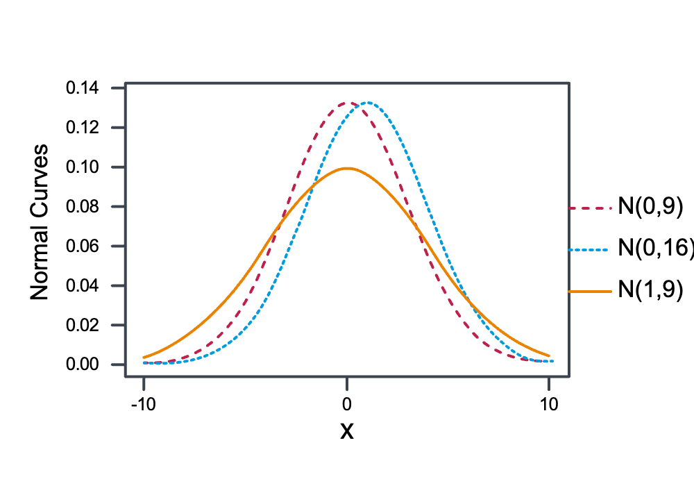
   Fig 16.1

   As claimed, the shapes of the three curves differ, as the means \(\mu\) and standard deviations \(\sigma\) differ.

16.2 Finding Normal Probabilities

Example 16.2 Let \(X\) equal the IQ of a randomly selected American. Assume \(X\sim N(100, 16^2)\).

What is the probability that a randomly selected American has an IQ below 90?

Solution

As is the case with all continuous distributions, finding the probability involves finding the area under the curve and to the left of the line \(x=90\):

Fig 16.2

That is:

\[ P(X \leq 90)=F(90)=\int^{90}_{-\infty} \dfrac{1}{16\sqrt{2\pi}}\text{exp}\left\{-\dfrac{1}{2}\left(\dfrac{x-100}{16}\right)^2\right\} dx \]

There’s just one problem… it is not possible to integrate the normal PDF That is, no simple expression exists for the antiderivative. We can only approximate the integral using numerical analysis techniques. So, all we need to do is find a normal probability table for a normal distribution with mean \(\mu=100\) and standard deviation \(\sigma=16\).

Aw, geez, there’d have to be an infinite number of normal probability tables. That strategy isn’t going to work! Aha! The cumulative probabilities have been tabled for the \(N(0,1)\) distribution. All we need to do is transform our \(N(100, 16^2)\) distribution to a \(N(0, 1)\) distribution and then use the cumulative probability table for the \(N(0,1)\) distribution to calculate our desired probability. The theorem that follows tells us how to make the necessary transformation.

NoteTheorem

If \(X\sim N(\mu, \sigma^2)\), then:

\[ Z=\dfrac{X-\mu}{\sigma} \]

follows the \(N(0,1)\) distribution, which is called the standardized (or standard) normal distribution.

Proof

We need to show that the random variable \(Z\) follows a \(N(0,1)\) distribution. So, let’s find the cumulative distribution function \(F(z)\), which is also incidentally referred to as \(\Phi(z)\) in the standard normal case (that’s the greek letter phi, read “fee”):

\[ F(z)=\Phi(z)=P(Z\leq z)=P \left(\dfrac{X-\mu}{\sigma} \leq z \right) \]

which, by rearranging and using the normal PDF, equals:

\[ F(z)=P(X\leq \mu+z\sigma)=\int^{\mu+z\sigma}_{-\infty} \dfrac{1}{\sigma \sqrt{2\pi}} \text{exp}\left\{-\dfrac{1}{2} \left(\dfrac{x-\mu}{\sigma}\right)^2\right\} \]

To perform the integration, let’s use the change of variable technique with:

\[ w=\dfrac{x-\mu}{\sigma} \]

so that:

\[ x = \sigma(w) + \mu \text{ and } dx = \sigma dw \]

Now for the endpoints of the integral: if \(x=-\infty\), then \(w\) also equals \(-\infty\); and if \(x=\mu+z\sigma\), then \(w=\frac{\mu+z\sigma -\mu}{\sigma}\). Therefore, upon making all of the substitutions for \(x, w\), and \(dx\), our integration looks like this:

\[ F(z)=\int^z_{-\infty}\dfrac{1}{\sigma \sqrt{2\pi}} \text{exp}\left\{-\dfrac{1}{2} w^2\right\} \sigma dw \]

And since the \(\sigma\) in the denominator cancels out the \(\sigma\) in the numerator, we get:

\[ F(z)=\int^z_{-\infty}\dfrac{1}{\sqrt{2\pi}} \text{exp}\left\{-\dfrac{1}{2} w^2\right\} dw \]

We should now recognize that as the cumulative distribution of a normal random variable with mean \(\mu=0\) and standard deviation \(\sigma=1\). Our proof is complete.

The theorem leads us to the following strategy for finding probabilities \(P(z<X<b)\) when \(a\) and \(b\) are constants, and \(X\) is a normal random variable with mean \(\mu\) and standard deviation \(\sigma\):

1. Specify the desired probability in terms of \(X\).

2. Transform \(X, a\), and \(b\), by:

   \[ Z=\dfrac{X-\mu}{\sigma} \]

3. Use the standard normal \(N(0,1)\) table, typically referred to as the \(Z\)-table, to find the desired probability.

Reading \(Z\)-tables

Standard normal, or \(Z\)-tables, can take a number of different forms. There are two standard normal tables, Table Va and Table Vb, in the back of our textbook. Table Va gives the cumulative probabilities for \(Z\)-values, to two decimal places, between 0.00 and 3.09. Here’s what the top of Table Va looks like:

Fig 16.3

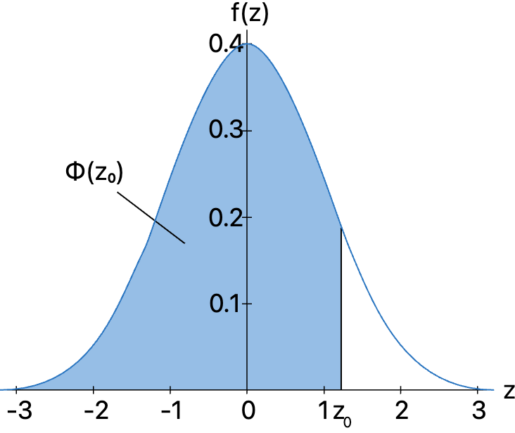
\[ \begin{align*} P(Z \leq z)&= \Phi(z)=\int_{-\infty}^{z} \frac{1}{\sqrt{2 \pi}} e^{-w^{2} / 2} dw \\ \Phi(-z) &=1-\Phi(z) \end{align*} \]

z	0.00	0.01	0.02	0.03	0.04	0.05	0.06	0.07	0.08	0.09
0.0	0.5000	0.5040	0.5080	0.5120	0.5160	0.5199	0.5239	0.5279	0.5319	0.5359
0.1	0.5398	0.5438	0.5478	0.5517	0.5557	0.5596	0.5636	0.5675	0.5714	0.5753
0.2	0.5793	0.5832	0.5871	0.5910	0.5948	0.5987	0.6026	0.6064	0.6103	0.6141
0.3	0.6179	0.6217	0.6255	0.6293	0.6310	0.6368	0.6406	0.6443	0.6480	0.6517
0.4	0.6554	0.6591	0.6628	0.6664	0.6700	0.6736	0.6772	0.6808	0.6844	0.6879

For example, you could use Table Va to find probabilities such as \(P(Z\le 0.01), P(Z\le 1.23)\), or \(P(Z\le 2.98)\). Table Vb, on the other hand, gives probabilities in the upper tail of the standard normal distribution. Here’s what the top of Table Vb looks like:

Fig 16.4

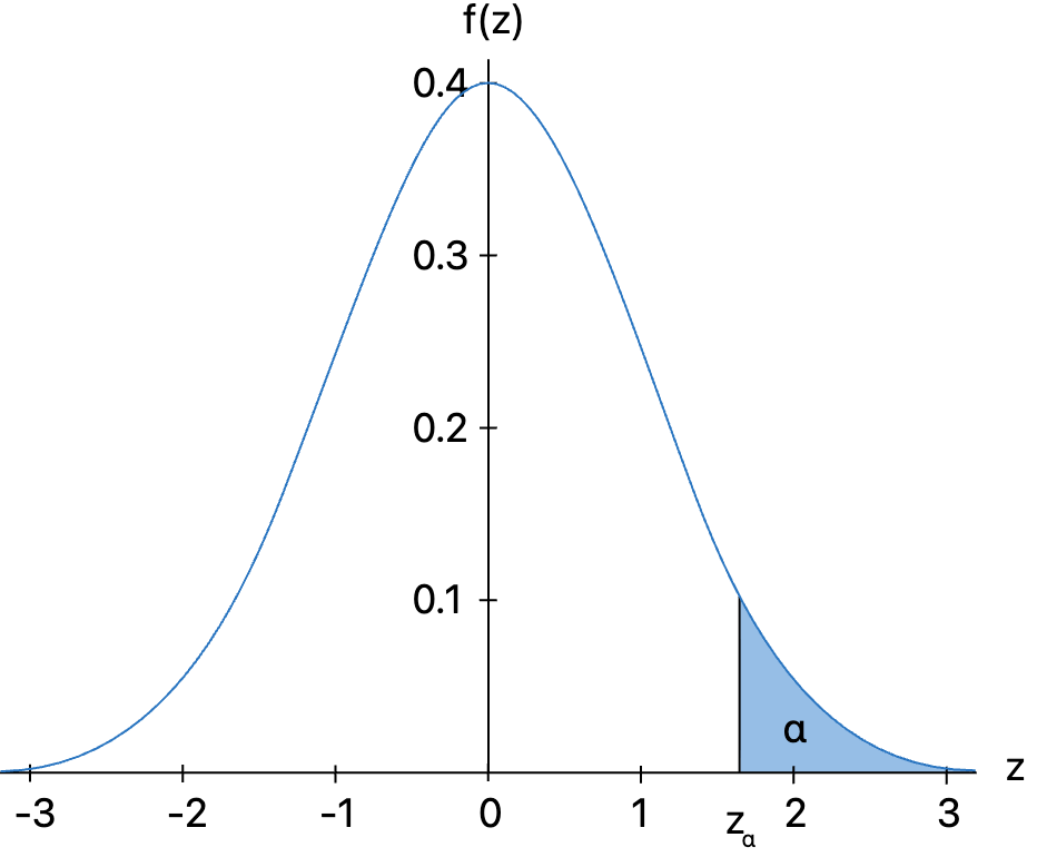
\[ P(Z > z_\alpha) = \alpha \]

\[ P(Z > z) = 1 - \Phi(z) = \Phi(-z) \]

\(z_\alpha\)	0.00	0.01	0.02	0.03	0.04	0.05	0.06	0.07	0.08	0.09
0.0	0.5000	0.4960	0.4920	0.4880	0.4840	0.4801	0.4761	0.4721	0.4681	0.4641
0.1	0.4602	0.4562	0.4522	0.4483	0.4443	0.4404	0.4364	0.4325	0.4286	0.4247
0.2	0.4207	0.4168	0.4129	0.4090	0.4520	0.4013	0.3974	0.3936	0.3897	0.3859
0.3	0.3821	0.3783	0.3745	0.3707	0.3669	0.3632	0.3594	0.3570	0.3557	0.3483
0.4	0.3446	0.3409	0.3372	0.3336	0.3300	0.3264	0.3228	0.3192	0.3192	0.3121

That is, for \(Z\)-values, to two decimal places, between 0.00 and 3.49, we can use Table Vb to find probabilities such as \(P(Z>0.12), P(Z>1.96)\), and \(P(Z>3.32)\).

Now, we just need to learn how to read the probabilities off of each of the tables. First Table Va:

Video 16.2: Example: The normal tables, part 1

And, then Table Vb:

Video 16.3: Example: The normal tables, part 2

Now we know how to read the given \(Z\)-tables. Now, we just need to work with some real examples to see that finding probabilities associated with a normal random variable usually involves rewriting the problems just a bit in order to get them to “fit” with the available \(Z\)-tables.

Example 16.3 Let \(X\) equal the IQ of a randomly selected American. Assume \(X\sim N(100, 16^2)\).

What is the probability that a randomly selected American has an IQ below 90?

Solution

Whenever I am faced with finding a normal probability, I always always always draw a picture of the probability I am trying to find. Then, the problem usually just solves itself… oh, how we wish:

Video 16.4: Example: An IQ below 90?

So, we just found that the desired probability, that is, that the probability that a randomly selected American has an IQ below 90 is 0.2643. (If you haven’t already, you might want to make sure that you can independently read that probability off of Table Vb.)

Now, although I used Table Vb in finding our desired probability, it is worth mentioning that I could have alternatively used Table Va. How’s that? Well:

\[ P(X<90)=P(Z<-0.63)=P(Z>0.63)=1-P(Z<0.63) \]

where the first equality comes from the transformation from \(X\) to \(Z\), the second equality comes from the symmetry of the normal distribution, and the third equality comes from the rule of complementary events. Using Table Va to look up \(P(Z<0.63)\), we get 0.7357. Therefore,

\[ P(X<90)=1-P(Z<0.63)=1-0.7357=0.2643 \]

We should, of course, be reassured that our logic produced the same answer regardless of the method used! That’s always a good thing!

What is the probability that a randomly selected American has an IQ above 140?

Solution

Again, I am going to solve this problem by drawing a picture:

Video 16.5: Example: An IQ above 140?

So, we just found that the desired probability, that is, that the probability that a randomly selected American has an IQ above 140 is 0.0062. (Again, if you haven’t already, you might want to make sure that you can independently read that probability off of Table Vb.)

We again could have alternatively used Table Va to find our desired probability:

\[ P(X>140)=P(Z>2.50)=1-P(Z<2.50 \]

where the first equality comes from the transformation from \(X\) to \(Z\), and the second equality comes from the rule of complementary events. Using Table Va to look up \(P(Z<2.5)\), we get 0.9938. Therefore,

\[ P(X>140)=1-P(Z<2.50)=1-0.9938=0.0062 \]

Again, we arrived at the same answer using two different methods.

What is the probability that a randomly selected American has an IQ between 92 and 114?

Solution

Again, I am going to solve this problem by drawing a picture:

Video 16.6: Example: An IQ between 92 and 114?

So, we just found that the desired probability, that is, that the probability that a randomly selected American has an IQ between 92 and 114 is 0.5021. (Again, if you haven’t already, you might want to make sure that you can independently read the probabilities that we used to get the answer from Tables Va and Vb.)

The previous three examples have illustrated each of the three possible normal probabilities you could be faced with finding —below some number, above some number, and between two numbers. Once you have mastered each case, then you should be able to find any normal probability when asked.

16.3 Using Normal Probabilities to Find X

On the last page, we learned how to use the standard normal curve N(0, 1) to find probabilities concerning a normal random variable X with mean \(\mu\) and standard deviation \(\sigma\). What happens if it’s not the probability that we want to find, but rather the value of X? That’s what we’ll investigate on this page. That is, we’ll consider what I like to call “inside-out” problems, in which we use known probabilities to find the value of the normal random variable X. Let’s start with an example.

Example 16.4 Suppose X, the grade on a midterm exam, is normally distributed with mean 70 and standard deviation 10. The instructor wants to give 15% of the class an A. What cutoff should the instructor use to determine who gets an A?

Solution

My approach to solving this problem is, of course, going to involve drawing a picture:

Video 16.7: Example: The 15% cutoff for an A grade?

The instructor now wants to give 10% of the class an A−.

What cutoff should the instructor use to determine who gets an A−?

Solution

We’ll use the same method as we did previously:

Video 16.8: Example: 10% of the class gets an A-?

In summary, in order to use a normal probability to find the value of a normal random variable X:

1. Find the z value associated with the normal probability.

2. Use the transformation \(x = \mu+ z \sigma\) to find the value of x.

16.4 Normal Properties

So far, all of our attention has been focused on learning how to use the normal distribution to answer some practical problems. We’ll turn our attention for a bit to some of the theoretical properties of the normal distribution. We’ll start by verifying that the normal PDF is indeed a valid probability distribution. Then, we’ll derive the moment-generating function \(M(t)\) of a normal random variable \(X\). We’ll conclude by using the moment-generating function to prove that the mean and standard deviation of a normal random variable \(X\) are indeed, respectively, \(\mu\) and \(\sigma\), something that we thus far have assumed without proof.

The Normal PDF is Valid

Recall that the probability density function of a normal random variable is:

\[ f(x)=\dfrac{1}{\sigma \sqrt{2\pi}} \text{exp}\left\{-\dfrac{1}{2} \left(\dfrac{x-\mu}{\sigma}\right)^2\right\} \]

for \(-\infty<x<\infty\), \(-\infty<\mu<\infty\), and \(0<\sigma<\infty\). Also recall that in order to show that the normal PDF is a valid PDF, we need to show that, firstly \(f(x)\) is always positive, and, secondly, if we integrate \(f(x)\) over the entire support, we get 1.

NoteProof

Let’s start with the easy part first, namely, showing that \(f(x)\) is always positive. The standard deviation \(\sigma\) is defined to be positive. The square root of \(2\pi\) is positive. And, the natural exponential function is positive. When you multiply positive terms together, you, of course, get a positive number. Check… the first part is done.

Now, for the second part. Showing that \(f(x)\) integrates to 1 is a bit messy, so bear with me here. Let’s define \(I\) to be the integral that we are trying to find. That is:

\[ I=\int_{-\infty}^\infty \dfrac{1}{\sigma \sqrt{2\pi}} \text{exp}\left\{-\dfrac{1}{2\sigma^2} (x-\mu)^2\right\}dx \]

Our goal is to show that \(I=1\). Now, if we change variables with:

\[ w=\dfrac{x-\mu}{\sigma} \]

our integral \(I\) becomes:

\[ I=\int_{-\infty}^\infty \dfrac{1}{\sqrt{2\pi}} \text{exp}\left\{-\dfrac{1}{2} w^2\right\}dw \]

Now, squaring both sides, we get:

\[ I^2=\left(\int_{-\infty}^\infty \dfrac{1}{\sqrt{2\pi}} \text{exp}\left\{-\dfrac{x^2}{2} \right\}dx\right) \left(\int_{-\infty}^\infty \dfrac{1}{\sqrt{2\pi}} \text{exp}\left\{-\dfrac{y^2}{2} \right\}dy\right) \]

And, pulling the integrals together, we get:

\[ I^2=\dfrac{1}{2\pi}\int_{-\infty}^\infty \int_{-\infty}^\infty \text{exp}\left\{-\dfrac{x^2}{2} \right\} \text{exp}\left\{-\dfrac{y^2}{2} \right\}dxdy \]

Now, combining the exponents, we get:

\[ I^2=\dfrac{1}{2\pi}\int_{-\infty}^\infty \int_{-\infty}^\infty \text{exp}\left\{-\dfrac{1}{2}(x^2+y^2) \right\} dxdy \]

Converting to polar coordinates with:

\[ x=r\cos\theta \text{ and } y=r\sin\theta \]

we get:

\[ I^2=\dfrac{1}{2\pi}\int_0^{2\pi}\left(\int_0^\infty \text{exp}\left\{-\dfrac{r^2}{2} \right\} rdr\right)d\theta \]

Now, if we do yet another change of variables with:

\[ u=\dfrac{r^2}{2} \text{ and } du=rdr \]

our integral \(I\) becomes:

\[ I^2=\dfrac{1}{2\pi}\int_0^{2\pi}\left(\int_0^\infty e^{-u}du\right)d\theta \]

Evaluating the inside integral, we get:

\[ I^2=\dfrac{1}{2\pi}\int_0^{2\pi}\left\{-\lim\limits_{b\to \infty} [e^{-u}]^{u=b}_{u=0}\right\}d\theta \]

And, finally, completing the integration, we get:

\[ I^2=\dfrac{1}{2\pi} \int_0^{2\pi} -(0-1) d \theta= \dfrac{1}{2\pi}\int_0^{2\pi} d \theta =\dfrac{1}{2\pi} (2\pi)=1 \]

Okay, so we’ve shown that \(I^2=1\). Therefore, that means that \(I=+1\) or \(I=-1\). But, we know that \(I\) must be positive, since \(f(x)>0\). Therefore, \(I\) must equal 1. Our proof is complete. Finally.

The Moment-Generating Function

NoteTheorem

The moment-generating function of a normal random variable \(X\) is:

\[ M(t)=\text{exp}\left\{\mu t+\dfrac{\sigma^2 t^2}{2}\right\} \]

Proof

Well, I better start this proof out by saying this one is a bit messy, too. Jumping right into it, using the definition of a moment-generating function, we get:

\[ M(t)=E(e^{tX})=\int_{-\infty}^\infty e^{tx}f(x)dx=\int_{-\infty}^\infty e^{tx}\left[\dfrac{1}{\sigma \sqrt{2\pi}} \text{exp}\left\{-\dfrac{1}{2\sigma^2} (x-\mu)^2\right\} \right]dx \]

Simply expanding the term in the second exponent, we get:

\[ M(t)=\int_{-\infty}^\infty \dfrac{1}{\sigma \sqrt{2\pi}}\text{exp}\{tx\} \text{exp}\left\{-\dfrac{1}{2\sigma^2} (x^2-2x\mu+\mu^2)\right\} dx \]

And, combining the two exponents, we get:

\[ M(t)=\int_{-\infty}^\infty \dfrac{1}{\sigma \sqrt{2\pi}} \text{exp}\left\{-\dfrac{1}{2\sigma^2} (x^2-2x\mu+\mu^2)+tx \right\} dx \]

Pulling the \(tx\) term into the parentheses in the exponent, we get:

\[ M(t)=\int_{-\infty}^\infty \dfrac{1}{\sigma \sqrt{2\pi}} \text{exp}\left\{-\dfrac{1}{2\sigma^2} (x^2-2x\mu-2\sigma^2tx+\mu^2) \right\} dx \]

And, simplifying just a bit more in the exponent, we get:

\[ M(t)=\int_{-\infty}^\infty \dfrac{1}{\sigma \sqrt{2\pi}} \text{exp}\left\{-\dfrac{1}{2\sigma^2} (x^2-2x(\mu+\sigma^2 t)+\mu^2) \right\} dx \]

And, simplifying just a bit more in the exponent, we get:

Now, let’s take a little bit of an aside by focusing our attention on just this part of the exponent:

\[ (x^2-2(\mu+\sigma^2t)x+\mu^2) \]

If we let:

\[ a=\mu+\sigma^2t \text{ and } b=\mu^2 \]

then that part of our exponent becomes:

\[ x^2-2(\mu+\sigma^2t)x+\mu^2=x^2-2ax+b \]

Now, complete the square by effectively adding 0:

\[ x^2-2(\mu+\sigma^2t)x+\mu^2=x^2-2ax+a^2-a^2+b \]

And, simplifying, we get:

\[ x^2-2(\mu+\sigma^2t)x+\mu^2=(x-a)^2-a^2+b \]

Now, inserting in the values we defined for \(a\) and \(b\), we get:

\[ x^2-2(\mu+\sigma^2t)x+\mu^2=(x-(\mu+\sigma^2t))^2-(\mu+\sigma^2t)^2+\mu^2 \]

Okay, now stick our modified exponent back into where we left off in our calculation of the moment-generating function:

\[ M(t)=\int_{-\infty}^\infty \dfrac{1}{\sigma \sqrt{2\pi}}\text{exp}\left\{-\dfrac{1}{2\sigma^2}\left[(x-(\mu+\sigma^2t))^2-(\mu+\sigma^2t)^2+\mu^2\right]\right\}dx \]

We can now pull the part of the exponent that doesn’t depend on \(x\) through the integral getting:

\[ M(t)=\text{exp}\left\{-\dfrac{1}{2\sigma^2}\left[-(\mu+\sigma^2t)^2+\mu^2\right]\right\} \int_{-\infty}^\infty \dfrac{1}{\sigma \sqrt{2\pi}}\text{exp}\left\{-\dfrac{1}{2\sigma^2}\left[(x-(\mu+\sigma^2t))^2 \right]\right\}dx \]

Now, we should recognize that the integral integrates to 1 because it is the integral over the entire support of the PDF of a normal random variable \(X\) with:

mean \(\mu+\sigma^2t\) and variance \(\sigma^2\)

That is, because the integral is 1:

\[ \int_{-\infty}^\infty \dfrac{1}{\sigma \sqrt{2\pi}}\text{exp}\left\{-\dfrac{1}{2\sigma^2}\left[(x-(\mu+\sigma^2t))^2 \right]\right\}dx = 1 \]

Since, \(N(\mu+\sigma^2t, \sigma^2)\).

our moment-generating function reduces to this:

\[ M(t)=\text{exp}\left\{-\dfrac{1}{2\sigma^2}\left[-\mu^2-2\mu\sigma^2t-\sigma^4t^2+\mu^2\right]\right\} \]

Now, it’s just a matter of simplifying:

\[ M(t)=\text{exp}\left\{\dfrac{2\mu\sigma^2t+\sigma^4t^2}{2\sigma^2}\right\} \]

and simplifying a bit more:

\[ M(t)=\text{exp}\left\{\mu t +\dfrac{\sigma^2t^2}{2}\right\} \]

Our second messy proof is complete!

The Mean and Variance

NoteTheorem

The mean and variance of a normal random variable \(X\) are, respectively, \(\mu\) and \(\sigma^2\).

Proof

We’ll use the moment-generating function:

\[ M(t)=\text{exp}\left\{\mu t +\dfrac{\sigma^2t^2}{2}\right\} \]

to find the mean and variance. Recall that finding the mean involves evaluating the derivative of the moment-generating function with respect to \(t\) at \(t=0\):

Video 16.9: Proof: The mean of a normal random variable X

So, we just found that the first derivative of the moment-generating function with respect to \(t\) is:

\[ M'(t)=\text{exp}\left(\mu t +\dfrac{\sigma^2t^2}{2}\right)\times (\mu+\sigma^2t) \]

We’ll use it to help us find the variance:

Video 16.10: Proof: The variance of a normal random variable X

16.5 The Standard Normal and The Chi-Square

NoteTheorem

We have one more theoretical topic to address before getting back to some practical applications on the next page, and that is the relationship between the normal distribution and the chi-square distribution. The following theorem clarifies the relationship.

If \(X\) is normally distributed with mean \(\mu\) and variance \(\sigma^2>0\), then:

\[ V=\left(\dfrac{X-\mu}{\sigma}\right)^2=Z^2 \]

is distributed as a chi-square random variable with 1 degree of freedom.

Proof

To prove this theorem, we need to show that the PDF of the random variable \(V\) is the same as the PDF of a chi-square random variable with 1 degree of freedom. That is, we need to show that:

\[ g(v)=\dfrac{1}{\Gamma(1/2)2^{1/2}}v^{\frac{1}{2}-1} e^{-v/2} \]

The strategy we’ll take is to find \(G(v)\), the cumulative distribution function of \(V\), and then differentiate it to get \(g(v)\), the probability density function of \(V\). That said, we start with the definition of the cumulative distribution function of \(V\):

\[ G(v)=P(V\leq v)=P(Z^2 \leq v) \]

That second equality comes, of course, from the fact that \(V=Z^2\). Now, taking note of the behavior of a parabolic function:

Fig 16.5

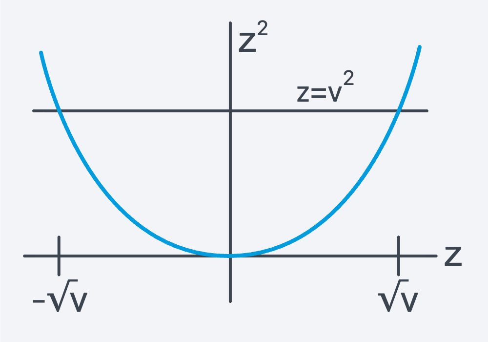
we can simplify \(G(v)\) to get:

\[ G(v)=P(-\sqrt{v} < Z <\sqrt{v}) \]

Now, to find the desired probability we need to integrate, over the given interval, the probability density function of a standard normal random variable \(Z\). That is:

\[ G(v)= \int^{\sqrt{v}}_{-\sqrt{v}}\dfrac{1}{ \sqrt{2\pi}}\text{exp} \left(-\dfrac{z^2}{2}\right) dz \]

By the symmetry of the normal distribution, we can integrate over just the positive portion of the integral, and then multiply by two:

\[ G(v)= 2\int^{\sqrt{v}}_0 \dfrac{1}{ \sqrt{2\pi}}\text{exp} \left(-\dfrac{z^2}{2}\right) dz \]

Okay, now let’s do the following change of variables:

Let \(\ z=\sqrt{y}=y^{1/2}\).

So, \(dz=\frac{1}{2}y^{-1/2}\ dy=\frac{1}{z\sqrt{y}}dy\)

\[ z^2=y, \begin{align*} z&=0 \Rightarrow y=0 \\ z&=\sqrt{v} \Rightarrow y=v\end{align*} \]

Doing so, we get:

\[ G(v)= 2\int^v_0 \dfrac{1}{ \sqrt{2\pi}}\text{exp} \left(-\dfrac{y}{2}\right) \left(\dfrac{1}{2\sqrt{y}}\right) dy \]

\[ G(v)= \int^v_0 \dfrac{1}{ \sqrt{\pi}\sqrt{2}} y^{\frac{1}{2}-1} \text{exp} \left(-\dfrac{y}{2}\right) dy \]

for \(v>0\). Now, by one form of the Fundamental Theorem of Calculus:

Given, \[ \int^x_a f(t)dt=F(x)-F(a) \]

\[ \frac{d}{dx}\int^x_a f(t)dt=F'(x)=f(x) \]

we can take the derivative of \(G(v)\) to get the probability density function \(g(v)\):

\[ g(v)=G'(v)= \dfrac{1}{ \sqrt{\pi}\sqrt{2}} v^{\frac{1}{2}-1} e^{-v/2} \]

for \(0<v<\infty\). If you compare this \(g(v)\) to the first \(g(v)\) that we said we needed to find way back at the beginning of this proof, you should see that we are done if the following is true:

\[ \Gamma \left(\dfrac{1}{2}\right)=\sqrt{\pi} \]

It is indeed true, as the following argument illustrates. Because \(g(v)\) is a PDF, the integral of the PDF over the support must equal 1:

\[ \int_0^\infty \dfrac{1}{ \sqrt{\pi}\sqrt{2}} v^{\frac{1}{2}-1} e^{-v/2} dv=1 \]

Now, change the variables by letting \(v=2x\), so that \(dv=2dx\). Making the change, we get:

\[ \dfrac{1}{ \sqrt{\pi}} \int_0^\infty \dfrac{1}{ \sqrt{2}} (2x)^{\frac{1}{2}-1} e^{-x}2dx=1 \]

Rewriting things just a bit, we get:

\[ \dfrac{1}{ \sqrt{\pi}} \int_0^\infty \dfrac{1}{ \sqrt{2}}\dfrac{1}{ \sqrt{2}} x^{\frac{1}{2}-1} e^{-x}2dx=1 \]

And simplifying, we get:

\[ \dfrac{1}{ \sqrt{\pi}} \int_0^\infty x^{\frac{1}{2}-1} e^{-x} dx=1 \]

Now, it’s just a matter of recognizing that the integral is the gamma function of \(\frac{1}{2}\):

\[ \dfrac{1}{ \sqrt{\pi}} \Gamma \left(\dfrac{1}{2}\right)=1 \]

Our proof is complete.

So, now that we’ve taken care of the theoretical argument. Let’s take a look at an example to see that the theorem is, in fact, believable in a practical sense.

Example 16.5 Find the probability that the standard normal random variable \(Z\) falls between −1.96 and 1.96 in two ways:

1. using the standard normal distribution
2. using the chi-square distribution

Solution

The standard normal table (Table V in the textbook) yields:

\[ \begin{align} P(-1.96<Z<1.96)&=P(Z<1.96)-P(Z>1.96)\\&=0.975-0.025\\&=0.95\end{align} \]

The chi-square table (Table IV in the textbook) yields the same answer:

\[ \begin{align} P(-1.96<Z<1.96)&=P(|Z|<1.96)\\&=P(Z^2<1.96^2)\\&=P(\chi^2_{(1)})<3.8416)\\&=0.95\end{align} \]

16.6 Some Applications

Interpretation of Z

Note that the transformation from \(X\) to \(Z\):

\[ Z=\dfrac{X-\mu}{\sigma} \]

tells us the number of standard deviations above or below the mean that \(X\) falls. That is, if \(Z=-2\), then we know that \(X\) falls 2 standard deviations below the mean. And if \(Z=+2\), then we know that \(X\) falls 2 standard deviations above the mean. As such, \(Z\)-scores are sometimes used in medical fields to identify whether an individual exhibits extreme values with respect to some biological or physical measurement.

Example 16.6

Post-menopausal women are known to be susceptible to severe bone loss known as osteoporosis. In some cases, bone loss can be so extreme as to cause a woman to lose a few inches of height. The spines and hips of women who are suspected of having osteoporosis are therefore routinely scanned to ensure that their bone loss hasn’t become so severe to warrant medical intervention.

The mean \(\mu\) and standard deviation \(\sigma\) of the density of the bones in the spine, for example, are known for a healthy population. A woman is scanned and \(x\), the bone density of her spine is determined. She and her doctor would then naturally want to know whether the woman’s bone density \(x\) is extreme enough to warrant medical intervention. The most common way of evaluating whether a particular \(x\) is extreme is to use the mean \(\mu\), the standard deviation \(\sigma\), and the value \(x\) to calculate a \(Z\)-score. The \(Z\)-score can then be converted to a percentile to provide the doctor and the woman an indication of the severity of her bone loss.

Suppose the woman’s \(Z\)-score is −2.36, for example. The doctor then knows that the woman’s bone density falls 2.36 standard deviations below the average bone density of a healthy population. The doctor, furthermore, knows that fewer than 1% of the population have a bone density more extreme than that of his/her patient.

The Empirical Rule Revisited

You might recall earlier in this section, when we investigated exploring continuous data, that we learned about the Empirical Rule. Specifically, we learned that if a histogram is at least approximately bell-shaped, then:

1. approximately 68% of the data fall within one standard deviation of the mean
2. approximately 95% of the data fall within two standard deviations of the mean
3. approximately 99.7% of the data fall within three standard deviations of the mean

Where did those numbers come from? Now, that we’ve got the normal distribution under our belt, we can see why the Empirical Rule holds true. The probability that a randomly selected data value from a normal distribution falls within one standard deviation of the mean is

\[ \begin{align} P(-1<Z<1)&=P(Z<1)-P(Z>1)\\&=0.8413-0.1587\\&=0.6826 \end{align} \]

That is, we should expect 68.26% (approximately 68%!) of the data values arising from a normal population to be within one standard deviation of the mean, that is, to fall in the interval:

\[ (\mu-\sigma, \mu+\sigma) \]

The probability that a randomly selected data value from a normal distribution falls within two standard deviations of the mean is

\[ \begin{align}P(-2<Z<2)&=P(Z<2)-P(Z>2)\\&=0.9772-0.0228\\&=0.9544\end{align} \]

That is, we should expect 95.44% (approximately 95%!) of the data values arising from a normal population to be within two standard deviations of the mean, that is, to fall in the interval:

\[ (\mu-2\sigma, \mu+2\sigma) \]

And, the probability that a randomly selected data value from a normal distribution falls within three standard deviations of the mean is:

\[ \begin{align}P(-3<Z<3)&=P(Z<3)-P(Z>3)\\&=0.9987-0.0013\\&=0.9974\end{align} \]

That is, we should expect 99.74% (almost all!) of the data values arising from a normal population to be within three standard deviations of the mean, that is, to fall in the interval:

\[ (\mu-3\sigma, \mu+3\sigma) \]

Let’s take a look at an example of the Empirical Rule in action.

Example 16.7 The left arm length, in inches, of 213 students were measured.

Here’s the resulting data,

Show Data

$$ \begin{array}{llllllllll} 25.5 & 21.0 & 25.5 & 25.5 & 23.5 & 26.5 & 30.0 & 20.5 & 25.5 & 26.0 \\ 26.0 & 22.5 & 24.0 & 27.0 & 24.5 & 23.0 & 24.5 & 26.5 & 24.0 & 24.1 \\ 24.0 & 28.0 & 23.0 & 27.0 & 26.5 & 24.5 & 26.0 & 23.0 & 22.0 & 21.5 \\ 26.0 & 24.0 & 26.0 & 25.5 & 23.0 & 25.5 & 24.0 & 24.0 & 29.0 & 25.0 \\ 24.0 & 25.5 & 24.0 & 24.1 & 26.0 & 25.5 & 24.5 & 24.5 & 24.5 & 22.5 \\ 26.5 & 26.5 & 25.5 & 26.5 & 30.5 & 25.0 & 24.0 & 23.0 & 24.5 & 24.0 \\ 25.5 & 26.5 & 24.0 & 24.5 & 29.5 & 26.5 & 24.0 & 24.0 & 25.0 & 23.5 \\ 23.4 & 24.5 & 24.5 & 29.0 & 27.0 & 23.3 & 29.0 & 21.5 & 22.5 & 28.0 \\ 23.5 & 28.0 & 28.6 & 23.0 & 28.0 & 25.0 & 25.0 & 24.0 & 23.0 & 28.0 \\ 31.0 & 25.0 & 25.5 & 24.0 & 26.7 & 27.0 & 24.0 & 27.0 & 25.5 & 23.5 \\ 29.5 & 22.9 & 25.0 & 28.0 & 25.0 & 23.5 & 28.0 & 26.5 & 21.5 & 22.0 \\ 25.4 & 25.0 & 26.2 & 28.0 & 22.5 & 23.0 & 26.1 & 23.4 & 27.0 & 25.5 \\ 26.0 & 29.0 & 25.4 & 25.5 & 25.5 & 25.5 & 24.5 & 25.0 & 22.0 & 30.5 \\ 23.0 & 23.0 & 25.5 & 27.5 & 27.0 & 22.5 & 23.5 & 28.0 & 22.2 & 26.0 \\ 24.5 & 25.5 & 22.0 & 25.4 & 23.5 & 23.0 & 23.5 & 24.0 & 22.0 & 21.5 \\ 23.5 & 27.0 & 25.5 & 23.5 & 24.8 & 23.0 & 27.0 & 25.0 & 24.0 & 24.6 \\ 30.0 & 28.0 & 25.0 & 26.0 & 25.4 & 23.5 & 25.0 & 24.0 & 29.0 & 23.5 \\ 28.0 & 26.0 & 25.0 & 21.0 & 27.0 & 27.0 & 24.0 & 25.0 & 25.5 & 28.0 \\ 24.9 & 23.5 & 27.2 & 30.0 & 23.0 & 23.0 & 24.0 & 24.0 & 21.0 & 24.0 \\ 25.0 & 28.0 & 24.0 & 25.4 & 25.0 & 22.0 & 25.5 & 22.5 & 29.0 & 25.5 \\ 25.0 & 27.0 & 26.0 & 25.5 & 29.0 & 28.5 & 24.5 & 22.5 & 26.5 & 28.0 \\ 24.6 & 24.5 & 27.5 \end{array} $$

…and a picture of a dot plot of the resulting arm lengths:

Fig 16.6

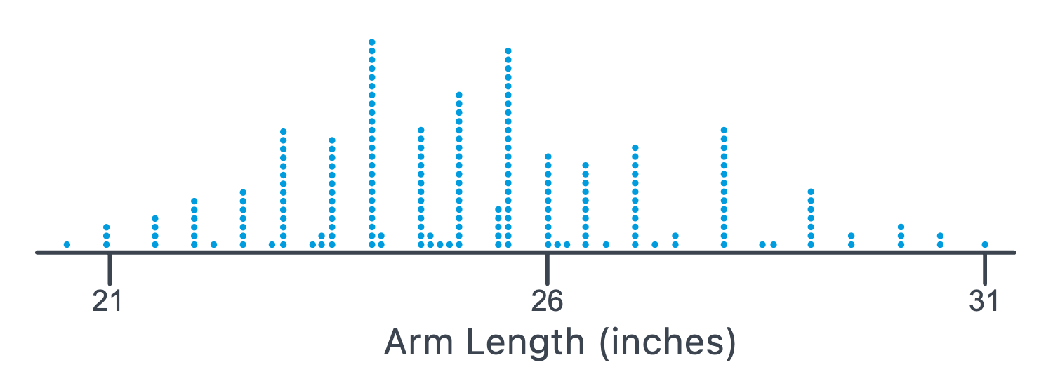
As you can see, the plot suggests that the distribution of the data is at least bell-shaped enough to warrant the assumption that \(X\), the left arm lengths of students, is normally distributed. We can use the raw data to determine that the average arm length of the 213 students measured is 25.167 inches, while the standard deviation is 2.095 inches. We’ll then use 25.167 as an estimate of \(\mu\), the average left arm length of all college students, and 2.095 as an estimate of \(\sigma\), the standard deviation of the left arm lengths of all college students.

The Empirical Rule tells us then that we should expect approximately 68% of all college students to have a left arm length between:

\[ \begin{align}\bar{x}-s=25.167-2.095=&23.072 \text{ and }\\ \bar{x}+s=25.167+2.095=&27.262\end{align} \]

inches. We should also expect approximately 95% of all college students to have a left arm length between:

\[ \begin{align}\bar{x}-2s=25.167-2(2.095)=&20.977 \text{ and }\\ \bar{x}+2s=25.167+2(2.095)=&29.357\end{align} \]

inches. And, we should also expect approximately 99.7% of all college students to have a left arm length between:

\[ \begin{align}\bar{x}-3s=25.167-3(2.095)=&18.882 \text{ and }\\ \bar{x}+3s=25.167+3(2.095)=&31.452\end{align} \]

Let’s see what percentage of our 213 arm lengths fall in each of these intervals! It takes some work if you try to do it by hand, but statistical software can quickly determine that:

• 143, or 67.14%, of the 213 arm lengths fall in the first interval
• 204, or 95.77%, of the 213 arm lengths fall in the second interval
• 213, or 100%, of the 213 arm lengths fall in the third interval

The Empirical Rule didn’t do too badly, eh?