Section 1: Introduction to Probability

In the lessons that follow, and throughout the rest of this course, we'll be learning all about the basics of probability — its properties, how it behaves, and how to calculate a probability. To do so, we'll be simultaneously working through this section, that is, Section 1, and the first chapter in the Hogg and Tanis textbook (10th edition).

Lesson 1: The Big Picture

Overview

In this lesson, our primary aim is to get a big picture of the entire course that lies ahead of us. Along the way, we'll also learn some basic concepts to help us begin to build our probability tool box.

Objectives

Upon completion of this lesson, you should be able to:

Learn the distinction between a population and a sample.
Learn how to define an outcome (sample) space.
Learn how to identify the different types of data: discrete, continuous, categorical, binary.
Learn how to summarize quantitative data graphically using a histogram.
Learn how statistical packages construct histograms for discrete data.
Learn how statistical packages construct histograms for continuous data.
Learn the distinction between frequency histograms, relative frequency histograms, and density histograms.
Learn how to "read" information from the three types of histograms.
Learn the big picture of the course, that is, put the material of sections 1 through 5 here on-line, and chapters 1 through 5 in the text, into a framework for the course.

1.1 - Some Research Questions

Research studies are conducted in order to answer some kind of research question(s). For example, the researchers in the Vegan Health Study define at least eight primary questions that they would like answered about the health of people who eat an entirely animal-free diet (no meat, no dairy, no eggs). Another research study was recently conducted to determine whether people who take the pain medications Vioxx or Celebrex are at a higher risk for heart attacks than people who don't take them. The list goes on. Researchers are working every day to answer their research questions.

What do you think about these research questions?

What percentage of college students feel sleep-deprived?
What is the probability that a randomly selected PSU student gets more than seven hours of sleep each night?
Do women typically cry more than men?
What is the typical number of credit cards owned by Stat 414 students?

Assuming that the above questions don't float your boat, can you formulate a few research questions that do interest you?

If we were to attempt to answer our research questions, we would soon learn that we couldn't ask every person in the population if they feel sleep-deprived, how often they cry, or the number of credit cards they have.

Try It!

How can we answer our research question if we can't ask every person in the population our research question?

We could take a random sample from the population, and use the resulting sample to learn something about the population.

1.2 - Populations and Random Samples

In trying to answer each of our research questions, whether yours or mine, we unfortunately can't ask every person in the population. Instead, we take a random sample from the population, and use the resulting sample to learn something, or make an inference, about the population:

For the research question "what percentage of college students feel sleep-deprived?", the population of interest is all college students. Therefore, assuming we are restricting the population to be U.S. college students, a random sample might consist of 1300 randomly selected students from all of the possible colleges in the United States. For the research question, "what is the probability that a randomly selected Penn State student gets more than 7 hours of sleep each night?", the population of interest is a little narrower, namely only Penn State students. In this case, a random sample might consist of, say, 300 randomly selected Penn State students. For the research question "what is the typical number of credit cards owned by Stat 414 students?", the population of interest is even more narrow, namely only the students enrolled in Stat 414. Ahhhh! If we are only interested in students currently enrolled in Stat 414, we have no need for taking a random sample. Instead, we can conduct a census, in which all of the students are polled.

Try It!

Identify the population and describe a potential random sample for the research question "do women typically cry more than men?"

The population is all women and all men, at least 18 years of age, perhaps. One possible sample is 50 randomly selected women and 50 randomly selected men.

Now, for each of the research questions you previously defined, identify the population of interest and describe a potential random sample.

The answers (or data) we get to our research questions of course depend on who ends up in our random sample. We can't possibly predict the possible outcomes with certainty, but we can at least create a list of possible outcomes.

1.3 - Sample Spaces

Sample Space: The sample space (or outcome space), denoted $\mathbf{S}$, is the collection of all possible outcomes of a random study.

In order to answer my first research question, we would need to take a random sample of U.S. college students, and ask each one "Do you feel sleep-deprived?" Each student should reply either "yes" or "no." Therefore, we would write the sample space as:

$\mathbf{S} = \{\text{yes}, \text{no}\}$

In order to answer my second research question, we would need to know how many hours of sleep a random sample of college students gets each night. One way of getting this information is to ask each selected student to record the number of hours of sleep they had last night. In this case, if we let h denote the number of hours slept, we would write the sample space as:

$\mathbf{S} = \{h: h \ge 0 \text{ hours}\}$

Hmmm, if we conducted a random study to answer my third research question, how would we define our sample space? Well, of course, it depends on how we went about trying to answer the question. If we asked a random sample of men and women "on how many days did you cry last month?", we would write the sample space as:

$\mathbf{S} = \{0, 1, 2, ..., 31\}$

Finally, if we were interested in learning about students who took Stat 414 in the past decade when trying to answer my fourth research question, we might ask all current Stat 414 students "how many credit cards do you have?" In that case, we would write our sample space as:

$\mathbf{S} = \{0, 1, 2, ...\}$

There is not always just one way of obtaining an answer to a research question. For my second research question, how would we define the sample space if we instead asked a random sample of college students "did you get more than seven hours of sleep last night?"

For each of the research questions you created:

Formulate the question you would ask (or describe the measurement technique you would use).
Define the resulting sample space.

Once we collect sample data, we need to do something with it. Like summarizing it would be good! How we summarize data depends on the type of data we collect.

1.4 - Types of data

Example 1-1

Your instructor asked a random sample of 20 college students "do you consider yourself to be sleep-deprived?" Their replies were:

yes	yes	yes	no	no	no	yes	yes	yes	yes
yes	no	no	yes	yes	no	yes	yes	yes	yes

Of course, it would be good to summarize the students' responses. What we do with the data though depends on the type of data collected. For our purposes, we will primarily be concerned with three types of data:

discrete
continuous
categorical

Now, for their definitions!

Discrete Data

Quantitative data are called discrete if the sample space contains a finite or countably infinite number of values.

Recall that a set of elements are countably infinite if the elements in the set can be put into one-to-one correspondence with the positive integers. My third research question yields discrete data, because of its sample space:

$\mathbf{S} = \{0, 1, 2, ..., 31\}$

contains a finite number of values. And, my fourth research question yields discrete data, because of its sample space:

$\mathbf{S} = \{0, 1, 2, ...\}$

contains a countably infinite number of values.

Continuous Data

Quantitative data are called continuous if the sample space contains an interval or continuous span of real numbers.

My second research question yields continuous data, because of its sample space:

$\mathbf{S} = \{h: h \ge 0 \text{ hours}\}$

is the entire positive real line. For continuous data, there is theoretically an infinite number of possible outcomes; the measurement tool is the restricting factor. For example, if I were to ask how much each student in the class weighed (in pounds), I would most likely get responses such as 126, 172, and 210. The responses are seemingly discrete. But, are they? If I report that I weigh 118 pounds, am I exactly 118 pounds? Probably not; I'm perhaps 118.0120980335927.... pounds. It's just that the scale that I get on in the morning tells me that I weigh 118 pounds. Again, the measurement tool is the restricting factor — something you always have to think about when trying to distinguish between discrete and continuous data.

Categorical Data

Qualitative data are called categorical if the sample space contains objects that are grouped or categorized based on some qualitative trait. When there are only two such groups or categories, the data are considered binary.

My first research question yields binary data because its sample space is:

$\mathbf{S} = \{\text{yes}, \text{ no}\}$

Two other examples of categorical data are eye color (brown, blue, hazel, and so on) and semester standing (freshman, sophomore, junior and senior).

1.5 - Summarizing Quantitative Data Graphically

Example 1-2

As discussed previously, how we summarize a set of data depends on the type of data. Let's take a look at an example. A sample of 40 female statistics students were asked how many times they cried in the previous month. Their replies were as follows:

9	5	3	2	6	3	2	2	3	4	2	8	4	4
5	0	3	0	2	4	2	1	1	2	2	1	3	0
2	1	3	0	0	2	2	3	4	1	1	5

That is, one student reported having cried nine times in the one month, while five students reported having cried not at all. It's pretty hard to draw too many conclusions about the frequency of crying for females statistics students without summarizing the data in some way.

Of course, a common way of summarizing such discrete data is by way of a histogram.

Here's what a frequency histogram of these data look like:

As you can see, a histogram gives a nice picture of the "distribution" of the data. And, in many ways, it's pretty self-explanatory. What are the notable features of the data? Well, the picture tells us:

The most common number of times that the women cried in the month was two (called the "mode").
The numbers ranged from 0 to 9 (that is, the "range" of the data is 9).
A majority of women (22 out of 40) cried two or fewer times, but a few cried as much as six or more times.

Can you think of anything else that the frequency histogram tells us? If we took another sample of 40 female students, would a frequency histogram of the new data look the same as the one above? No, of course not — that's what variability is all about.

Can you create a series of steps that a person would have to take in order to make a frequency histogram such as the one above? Does the following set of steps seem reasonable?

To create a frequency histogram of (finite) discrete data

Determine the number, $n$, in the sample.
Determine the frequency, $f_i$, of each outcome $i$.
Center a rectangle with base of length 1 at each observed outcome $i$ and make the height of the rectangle equal to the frequency.

For our crying (out loud) data, we would first tally the frequency of each outcome:


# OF TIMES	Tally	Frequency $f_i$
0	\|\|\|\|\|	5
1	\|\|\|\|\| \|	6
2	\|\|\|\|\| \|\|\|\|\| \|	11
3	\|\|\|\|\| \|\|	7
4	\|\|\|\|\|	5
5	\|\|\|	3
6	\|	1
7		0
8	\|	1
9	\|	1
		$n$=40

and then we'd use the first column for the horizontal-axis and the third column for the vertical-axis to draw our frequency histogram:

Well, of course, in practice, we'll not need to create histograms by hand. Instead, we'll just let statistical software (such as Minitab) create histograms for us.

Okay, so let's use the above frequency histogram to answer a few more questions:

What percentage of the surveyed women reported not crying at all in the month?
What percentage of the surveyed women reported crying two times in the month? and three times?

Clearly, the frequency histogram is not a 100%-user friendly. To answer these types of questions, it would be better to use a relative frequency histogram:

Now, the answers to the questions are a little more obvious — about 12% reported not crying at all; about 28% reported crying two times; and about 18% reported crying three times.

To create a relative frequency histogram of (finite) discrete data

Determine the number, $n$, in the sample.
Determine the frequency, $f_i$, of each outcome $i$.
Calculate the relative frequency (proportion) of each outcome $i$ by dividing the frequency of outcome $i$ by the total number in the sample $n$ — that is, calculate $\frac{f_i}{n}$ for each outcome $i$.
Center a rectangle with base of length 1 at each observed outcome i and make the height of the rectangle equal to the relative frequency.

While using a relative frequency histogram to summarize discrete data is a worthwhile pursuit in and of itself, my primary motive here in addressing such histograms is to motivate the material of the course. In our example, if we

let X = the number of times (days) a randomly selected student cried in the last month, and
let x = 0, 1, 2, ..., 31 be the possible values

Then $h_0=\frac{f_0}{n}$ is the relative frequency (or proportion) of students, in a sample of size $n$, crying $x_0$ times. You can imagine that for really small samples $\frac{f_0}{n}$ is quite unstable (think $n = 5$, for example). However, as the sample size $n$ increases, $\frac{f_0}{n}$ tends to stabilize and approach some limiting probability $p_0=f(x_0)$ (think $n = 1000$, for example). You can think of the relative frequency histogram serving as a sample estimate of the true probabilities of the population.

It is this $f(x_0)$, called a (discrete) probability mass function, that will be the focus of our attention in Section 2 of this course.

Example 1-3

Let's take a look at another example. The following numbers are the measured nose lengths (in millimeters) of 60 students:

38	50	38	40	35	52	45	50	40	32	40	47	70	55	51
43	40	45	45	55	37	50	45	45	55	50	45	35	52	32
45	50	40	40	50	41	41	40	40	46	45	40	43	45	42
45	45	48	45	45	35	45	45	40	45	40	40	45	35	52

How would we create a histogram for these data? The numbers look discrete, but they are technically continuous. The measuring tools, which consisted of a piece of string and a ruler, were the limiting factors in getting more refined measurements. Do you also notice that, in most cases, nose lengths come in five-millimeter increments... 35, 40, 45, 55...? Of course not, silly me... that's, again, just measurement error. In any case, if we attempted to use the guidelines for creating a histogram for discrete data, we'd soon find that the large number of disparate outcomes would prevent us from creating a meaningful summary of the data. Let's instead follow these guidelines:

To create a histogram of continuous data (or discrete data with many possible outcomes)

The major difference is that you first have to group the data into a set of classes, typically of equal length. There are many, many sets of rules for defining the classes. For our purposes, we'll just rely on our common sense — having too few classes is as bad as having too many.

Determine the number, $n$, in the sample.
Define $k$ class intervals $(c_0, c_1], (c_1, c_2], ..., (c_{k-1}, c_k]$.
Determine the frequency, $f_i$, of each class $i$.
Calculate the relative frequency (proportion) of each class by dividing the class frequency by the total number in the sample — that is, $\frac{f_i}{n}$.
For a frequency histogram: draw a rectangle for each class with the class interval as the base and the height equal to the frequency of the class.
For a relative frequency histogram: draw a rectangle for each class with the class interval as the base and the height equal to the relative frequency of the class.
For a density histogram: draw a rectangle for each class with the class interval as the base and the height equal to $h(x)=\dfrac{f_i}{n(c_i-c_{i-1})}$ for $c_{i-1}<x \leq c_i$, $i = 1, 2,..., k$.

Here's what the work would like for our nose length example if we used 5 mm classes centered at 30, 35, ... 70:


Class Interval	Tally	Frequency	Relative Frequency	Density Height
27.5-32.5	\|\|	2	0.033	0.0066
32.5-37.5	\|\|\|\|\|	5	0.083	0.0166
37.5-42.5	\|\|\|\|\| \|\|\|\|\| \|\|\|\|\| \|\|	17	0.283	0.0566
42.5-47.5	\|\|\|\|\| \|\|\|\|\| \|\|\|\|\| \|\|\|\|\| \|	21	0.350	0.0700
47.5-52.5	\|\|\|\|\| \|\|\|\|\| \|	11	0.183	0.0366
52.5-57.5	\|\|\|	3	0.183	0.0366
57.5-62.5		0	0	0
62.5-67.5		0	0	0
67.5-72.5	\|	1	0.017	0.0034
		60	0.999 (rounding)

For example, the relative frequency for the first class (27.5 to 32.5) is 2/60 or 0.033, whereas the height of the rectangle for the first class in a density histogram is 0.033/5 or 0.0066. Here is what the density histogram would like in its entirety:

Note that a density histogram is just a modified relative frequency histogram. That is, a density histogram is defined so that:

the area of each rectangle equals the relative frequency of the corresponding class, and
the area of the entire histogram equals 1.

Again, while using a density histogram to summarize continuous data is a worthwhile pursuit in and of itself, my primary motive here in addressing such histograms is to motivate the material of the course. As the sample size $n$ increases, we can imagine our density histogram approaching some limiting continuous function $f(x)$, say. It is this continuous curve $f(x)$ that we will come to know in Section 3 as a (continuous) probability density function.

So, in Section 2, we'll learn about discrete probability mass functions (p.m.f.s). In Section 3, we'll learn about continuous probability density functions (p.d.f.s). In Section 4, we'll learn about p.m.f.s and p.d.f.s for two (random) variables (instead of one). In Section 5, we'll learn how to find the probability distribution for functions of two or more (random) variables. Wow! That's a lot of work. Before we can take it on, however, we will first spend some time in this Section 1 filling up our probability toolbox with some basic probability rules and tools.

Lesson 2: Properties of Probability

Overview

In this lesson, we learn the fundamental concepts of probability. It is this lesson that will allow us to start putting our first tools into our new probability toolbox.

Objectives

Upon completion of this lesson, you should be able to:

Learn why an understanding of probability is so critically important to the advancement of most kinds of scientific research.
Learn the definition of an event.
Learn how to derive new events by taking subsets, unions, intersections, and/or complements of already existing events.
Learn the definitions of specific kinds of events, namely empty events, mutually exclusive (or disjoint) events, and exhaustive events.
Learn the formal definition of probability.
Learn three ways — the person opinion approach, the relative frequency approach, and the classical approach — of assigning a probability to an event.
Learn five fundamental theorems, which when applied, allow us to determine probabilities of various events.
Get lots of practice calculating probabilities of various events.

2.1 - Why Probability?

In the previous lesson, we discussed the big picture of the course without really delving into why the study of probability is so vitally important to the advancement of science. Let's do that now by looking at two examples.

Example 2-1

Suppose that the Penn State Committee for the Fun of Students claims that the average number of concerts attended yearly by Penn State students is 2. Then, suppose that we take a random sample of 50 Penn State students and determine that the average number of concerts attended by the 50 students is:

$\dfrac{1+4+3+\ldots+2}{50}=3.2$

that is, 3.2 concerts per year. That then begs the question: if the actual population average is 2, how likely is it that we'd get a sample average as large as 3.2?

What do you think? Is it likely or not likely? If the answer to the question is ultimately "not likely", then we have two possible conclusions:

Either: The true population average is indeed 2. We just happened to select a strange and unusual sample.
Or: Our original claim of 2 is wrong. Reject the claim, and conclude that the true population average is more than 2.

Of course, I don't raise this example simply to draw conclusions about the frequency with which Penn State students attend concerts. Instead I raise it to illustrate that in order to use a random sample to draw a conclusion about a population, we need to be able to answer the question "how likely...?", that is "what is the probability...?". Let's take a look at another example.

Example 2-2

Suppose that the Penn State Parking Office claims that two-thirds (67%) of Penn State students maintain a car in State College. Then, suppose we take a random sample of 100 Penn State students and determine that the proportion of students in the sample who maintain a car in State College is:

$\dfrac{69}{100}=0.69$

that is, 69%. Now we need to ask the question: if the actual population proportion is 0.67, how likely is it that we'd get a sample proportion of 0.69?

What do you think? Is it likely or not likely? If the answer to the question is ultimately "likely," then we have just one possible conclusion: The Parking Office's claim is reasonable. Do not reject their claim.

Again, I don't raise this example simply to draw conclusions about the driving behaviors of Penn State students. Instead I raise it to illustrate again that in order to use a random sample to draw a conclusion about a population, we need to be able to answer the question "how likely...?", that is "what is the probability...?".

Summary

So, in summary, why do we need to learn about probability? Any time we want to answer a research question that involves using a sample to draw a conclusion about some larger population, we need to answer the question "how likely is it...?" or "what is the probability...?". To answer such a question, we need to understand probability, probability rules, and probability models. And that's exactly what we'll be working on learning throughout this course.

Now that we've got the motivation for this probability course behind us, let's delve right in and start filling up our probability tool box!

2.2 - Events

Recall that given a random experiment, then the outcome space (or sample space) $\mathbf{S}$ is the collection of all possible outcomes of the random experiment.

Event: denoted with capital letters $A, B, C$, ... — is just a subset of the sample space $\mathbf{S}$. That is, for example $A\subset \mathbf{S}$, where "$\subset$" denotes "is a subset of."

Example 2-3

Suppose we randomly select a student, and ask them "how many pairs of jeans do you own?". In this case our sample space $\mathbf{S}$ is:

$\mathbf{S} = \{0, 1, 2, 3, ...\}$

We could theoretically put some realistic upper limit on that sample space, but who knows what it would be? So, let's leave it as accurate as possible. Now let's define some events.

If $A$ is the event that a randomly selected student owns no jeans:

$A$ = student owns none = $\{0\}$

If $B$ is the event that a randomly selected student owns some jeans:

$B$ = student owns some = $\{1, 2, 3, ...\}$

If $C$ is the event that a randomly selected student owns no more than five pairs of jeans:

$C$ = student owns no more than five pairs = $\{0, 1, 2, 3, 4, 5\}$

And, if $D$ is the event that a randomly selected student owns an odd number of pairs of jeans:

$D$ = student owns an odd number = $\{1, 3, 5, ...\}$

Review

Since events and sample spaces are just sets, let's review the algebra of sets:

$\emptyset$ is the "null set" (or "empty set")
$C\cup D$ = "union" = the elements in $C$ or $D$ or both
$A\cap B$ = "intersection" = the elements in $A$ and $B$. If (A\cap B=\emptyset\), then $A$ and $B$ are called "mutually exclusive events" (or "disjoint events").
$D^\prime=D^c$= "complement" = the elements not in $D$
If $E\cup F\cup G...=\mathbf{S}$, then $E, F, G$, and so on are called "exhaustive events."

Example 2-3 Continued

Let's revisit the previous "how many pairs of jeans do you own?" example. That is, suppose we randomly select a student, and ask them "how many pairs of jeans do you own?". In this case our sample space S is:

$\mathbf{S} = \{0, 1, 2, 3, ...\}$

Now, let's define some composite events.

The union of events $C$ and $D$ is the event that a randomly selected student either owns no more than five pairs or owns an odd number. That is:

$C\cup D=\{0, 1, 2, 3, 4, 5, 7, 9, ...\}$

The intersection of events $A$ and $B$ is the event that a randomly selected student owes no pairs and owes some pairs of jeans. That is:

$A\cap B = \{0\} \cap \{1, 2, 3, ...\}$ = the empty set $\emptyset$

The complement of event $D$ is the event that a randomly selected student owes an even number of pairs of jeans. That is:

$D^\prime= \{0, 2, 4, 6, ...\}$

If $E = \{0, 1\}$, $F = \{2, 3\}$, $G = \{4, 5\}$ and so on, so that:

$E\cup F\cup G\cup ...=\mathbf{S}$

then $E, F, G$, and so on are exhaustive events.

2.3 - What is Probability (Informally)?

We'll get to the more formal definition of probability soon, but let's think about probability just informally for a moment. How about this as an informal definition?

Probability: a number between 0 and 1; a number closer to 0 means "not likely"; a number closer to 1 means "quite likely"; If the probability of an event is exactly 0, then the event can't occur. If the probability of an event is exactly 1, then the event will definitely occur.

Try It!

Can you think of an event that cannot occur? Can you think of an event that will definitely occur?

An example of an event that can’t occur is rolling a seven from a fair six-sided die with face values {1, 2, 3, 4, 5, 6}. An example of an event that will definitely occur is the sun setting tonight.

2.4 - How to Assign Probability to Events

We know that probability is a number between 0 and 1. How does an event get assigned a particular probability value? Well, there are three ways of doing so:

the personal opinion approach
the relative frequency approach
the classical approach

On this page, we'll take a look at each approach.

The Personal Opinion Approach

This approach is the simplest in practice, but therefore it also the least reliable. You might think of it as the "whatever it is to you" approach. Here are some examples:

"I think there is an 80% chance of rain today."
"I think there is a 50% chance that the world's oil reserves will be depleted by the year 2100."
"I think there is a 1% chance that the men's basketball team will end up in the Final Four sometime this decade."

Example 2-4

At which end of the probability scale would you put the probability that:

one day you will die?
you can swim around the world in 30 hours?
you will win the lottery someday?
a randomly selected student will get an A in this course?
you will get an A in this course?

Answer

I think we'd all agree that the probability that you will die one day is 1. On the other hand, the probability that you can swim around the world in 30 hours is nearly 0, as is the probability that you will win the lottery someday. I am going to say that the probability that a randomly selected student will get an A in this course is a probability in the 0.20 to 0.30 range. I'll leave it to you think about the probability that you will get an A in this course.

The Relative Frequency Approach

The relative frequency approach involves taking the follow three steps in order to determine P(A), the probability of an event A:

Perform an experiment a large number of times, n, say.
Count the number of times the event A of interest occurs, call the number N(A), say.
Then, the probability of event A equals:

$P(A)=\dfrac{N(A)}{n}$

The relative frequency approach is useful when the classical approach that is described next can't be used.

Example 2-5

When you toss a fair coin with one side designated as a "head" and the other side designated as a "tail", what is the probability of getting a head?

Answer

I think you all might instinctively reply $\dfrac{1}{2}$. Of course, right? Well, there are three people who once felt compelled to determine the probability of getting a head using the relative frequency approach:

Coin Tosser	n, the number of tosses made	N(H), the number of heads tossed	P(H>)
Count Buffon	4,040	2,048	0.5069
Karl Pearson	24,000	12,012	0.5005
John Kerrich	10,000	5,067	0.5067

As you can see, the relative frequency approach yields a pretty good approximation to the 0.50 probability that we would all expect of a fair coin. Perhaps this example also illustrates the large number of times an experiment has to be conducted in order to get reliable results when using the relative frequency approach.

By the way, Count Buffon (1707-1788) was a French naturalist and mathematician who often pondered interesting probability problems. His most famous question

Suppose we have a floor made of parallel strips of wood, each the same width, and we drop a needle onto the floor. What is the probability that the needle will lie across a line between two strips?

came to be known as Buffon's needle problem. Karl Pearson (1857-1936) effectively established the field of mathematical statistics. And, once you hear John Kerrich's story, you might understand why he, of all people, carried out such a mind-numbing experiment. He was an English mathematician who was lecturing at the University of Copenhagen when World War II broke out. He was arrested by the Germans and spent the war interned in a prison camp in Denmark. To help pass the time he performed a number of probability experiments, such as this coin-tossing one.

Example 2-6

Some trees in a forest were showing signs of disease. A random sample of 200 trees of various sizes was examined yielding the following results:

Type	Disease free	Doubtful	Diseased	Total
Large	35	18	15	68
Medium	46	32	14	92
Small	24	8	8	40
Total	105	58	37	200

What is the probability that one tree selected at random is large?

Answer

There are 68 large trees out of 200 total trees, so the relative frequency approach would tell us that the probability that a tree selected at random is large is 68/200 = 0.34.

What is the probability that one tree selected at random is diseased?

Answer

There are 37 diseased trees out of 200 total trees, so the relative frequency approach would tell us that the probability that a tree selected at random is diseased is 37/200 = 0.185.

What is the probability that one tree selected at random is both small and diseased?

Answer

There are 8 small, diseased trees out of 200 total trees, so the relative frequency approach would tell us that the probability that a tree selected at random is small and diseased is 8/200 = 0.04.

What is the probability that one tree selected at random is either small or disease-free?

Answer

There are 121 trees (35 + 46 + 24 + 8 + 8) out of 200 total trees that are either small or disease-free, so the relative frequency approach would tell us that the probability that a tree selected at random is either small or disease-free is 121/200 = 0.605.

What is the probability that one tree selected at random from the population of medium trees is doubtful of disease?

Answer

There are 92 medium trees in the sample. Of those 92 medium trees, 32 have been identified as being doubtful of disease. Therefore, the relative frequency approach would tell us that the probability that a medium tree selected at random is doubtful of disease is 32/92 = 0.348.

The Classical Approach

The classical approach is the method that we will investigate quite extensively in the next lesson. As long as the outcomes in the sample space are equally likely (!!!), the probability of event $A$ is:

$P(A)=\dfrac{N(A)}{N(\mathbf{S})}$

where $N(A)$ is the number of elements in the event $A$, and $N(\mathbf{S})$ is the number of elements in the sample space $\mathbf{S}$. Let's take a look at an example.

Example 2-7

Suppose you draw one card at random from a standard deck of 52 cards. Recall that a standard deck of cards contains 13 face values (Ace, 2, 3, 4, 5, 6, 7, 8, 9, 10, Jack, Queen, and King) in 4 different suits (Clubs, Diamonds, Hearts, and Spades) for a total of 52 cards. Assume the cards were manufactured to ensure that each outcome is equally likely with a probability of 1/52. Let $A$ be the event that the card drawn is a 2, 3, or 7. Let $B$ be the event that the card is a 2 of hearts (H), 3 of diamonds (D), 8 of spades (S) or king of clubs (C). That is:

$A= \{x: x \text{ is a }2, 3,\text{ or }7\}$
$B = \{x: x\text{ is 2H, 3D, 8S, or KC}\}$

Then:

What is the probability that a 2, 3, or 7 is drawn?
What is the probability that the card is a 2 of hearts, 3 of diamonds, 8 of spades or king of clubs?
What is the probability that the card is either a 2, 3, or 7 or a 2 of hearts, 3 of diamonds, 8 of spades or king of clubs?
What is $P(A\cap B)$?

Answer

2.5 - What is Probability (Formally)?

Previously, we defined probability informally. Now, let's take a look at a formal definition using the “axioms of probability.”

Probability of the Event

Probability is a (real-valued) set function $P$ that assigns to each event $A$ in the sample space $\mathbf{S}$ a number $P(A)$, called the probability of the event $A$, such that the following hold:

The probability of any event $A$ must be nonnegative, that is, $P(A)\ge 0$.
The probability of the sample space is 1, that is, $P(\mathbf{S})=1$.
Given mutually exclusive events $A_1, A_2, A_3, ...$ that is, where $A_i\cap A_j=\emptyset$, for $i\ne j$,
$P(A_1\cup A_2 \cup \cdots \cup A_k)=P(A_1)+P(A_2)+\cdots+P(A_k)$

$P(A_1\cup A_2 \cup \cdots )=P(A_1)+P(A_2)+\cdots $
1. the probability of a finite union of the events is the sum of the probabilities of the individual events, that is:
2. the probability of a countably infinite union of the events is the sum of the probabilities of the individual events, that is:

Example 2-8

Suppose that a Stat 414 class contains 43 students, such that 1 is a Freshman, 4 are Sophomores, 20 are Juniors, 9 are Seniors, and 9 are Graduate students:

Status	Fresh	Soph	Jun	Sen	Grad	Total
Count	1	4	20	9	9	43
Proportion	0.02	0.09	0.47	0.21	0.21

Randomly select one student from the Stat 414 class. Defining the following events:

Fr = the event that a Freshman is selected
So = the event that a Sophomore is selected
Ju = the event that a Junior is selected
Se = the event that a Senior is selected
Gr = the event that a Graduate student is selected

The sample space is S = (Fr, So, Ju, Se, Gr}. Using the relative frequency approach to assigning probability to the events:

P(Fr) = 0.02
P(So) = 0.09
P(Ju) = 0.47
P(Se) = 0.21
P(Gr) = 0.21

Let's check to make sure that each of the three axioms of probability are satisfied.

2.6 - Five Theorems

Now, let's use the axioms of probability to derive yet more helpful probability rules. We'll work through five theorems in all, in each case first stating the theorem and then proving it. Then, once we've added the five theorems to our probability tool box, we'll close this lesson by applying the theorems to a few examples.

Theorem #1: $P(A)=1-P(A^\prime)$

Theorem #2.: $P(\emptyset)=0$

Theorem #3: If events $A$ and $B$ are such that $A\subseteq B$, then $P(A)\le P(B)$.

Theorem #4: $P(A)\le 1$

Theorem #5: For any two events $A$ and $B$, $P(A\cup B)=P(A)+P(B)-P(A\cap B)$.

2.7 - Some Examples

Example 2-9

A company has bid on two large construction projects. The company president believes that the probability of winning the first contract is 0.6, the probability of winning the second contract is 0.4, and the probability of winning both contracts is 0.2.

What is the probability that the company wins at least one contract?
What is the probability that the company wins the first contract but not the second contract?
What is the probability that the company wins neither contract?
What is the probability that the company wins exactly one contract?

Example 2-10

If it is known that $A\subseteq B$, what can be definitively said about $P(A\cap B)$?

Example 2-11

If 7% of the population smokes cigars, 28% of the population smokes cigarettes, and 5% of the population smokes both, what percentage of the population smokes neither cigars nor cigarettes?

Lesson 3: Counting Techniques

Overview

In the previous lesson, we learned that the classical approach to assigning probability to an event involves determining the number of elements in the event and the sample space. There are many situations in which it would be too difficult and/or too tedious to list all of the possible outcomes in a sample space. In this lesson, we will learn various ways of counting the number of elements in a sample space without actually having to identify the specific outcomes. The specific counting techniques we will explore include the multiplication rule, permutations and combinations.

Objectives

Upon completion of this lesson, you should be able to:

Understand and be able to apply the multiplication principle.
Understand how to count objects when the objects are sampled with replacement.
Understand how to count objects when the objects are sampled without replacement.
Understand and be able to use the permutation formula to count the number of ordered arrangements of $n$ objects taken $n$ at a time.
Understand and be able to use the permutation formula to count the number of ordered arrangements of $n$ objects taken $r$ at a time.
Understand and be able to use the combination formula to count the number of unordered subsets of $r$ objects taken from $n$ objects.
Understand and be able to use the combination formula to count the number of distinguishable permutations of $n$ objects, in which $r$ are of the objects are of one type and $n-r$ are of another type.
Understand and be able to count the number of distinguishable permutations of $n$ objects, when the objects are of more than two types.
Learn to apply the techniques learned in the lesson to new counting problems.

3.1 - The Multiplication Principle

Example 3-1

Dr. Roll Toss wants to calculate the probability that he will get:

a 6 6 on a die and a head penny

when he rolls a fair six-sided die and tosses a fair coin. Because his die is fair, he has an equally likely chance of getting any of the numbers 1, 2, 3, 4, 5, or 6. Similarly, because his coin is fair, he has an equally likely chance of getting a head or a tail. Therefore, he can use the classical approach of assigning probability to his event of interest. The probability of his event $A$, say, is:

$P(A)=\dfrac{N(A)}{N(S)}$

where $N(A)$ is the number of ways that he can get a 6 and a head, and $N(\mathbf{S})$ is the number of all of the possible outcomes of his rolls and tosses. There is of course only one possible way of getting a 6 and a head. Therefore, $N(A)$ is simply 1. To determine $N(\mathbf{S})$, he could enumerate all of the possible outcomes:

$\mathbf{S}=\{1H, 1T, 2H, 2T, \ldots\}$

and then count them up. Alternatively, he could use what is called the Multiplication Principle and recognize that for each of the 2 possible outcomes of a tossing a coin, there are exactly 6 possible outcomes of rolling a die. Therefore, there must be $6(2)=12$ possible outcomes in the sample space. The following animation illustrates the Multiplication Principle in action for Dr. Roll Toss' problem:

In summary, then the probability of interest here is $P(A)=\frac{1}{12}=0.083$. Of course, this example in itself is not particularly motivating. The main takeaway point should be that the Multiplication Principle exists and can be extremely useful for determining the number of outcomes of an experiment (or procedure), especially in situations when enumerating all of the possible outcomes of an experiment (procedure) is time- and/or cost-prohibitive. Let's generalize the principle.

Multiplication Principle: If there are:
$n_1$ outcomes of a random experiment $E_1$; $n_2$ outcomes of a random experiment $E_2$; ... and ...; $n_m$ outcomes of a random experiment $E_m$; then there are $n_1\times n_2\times\ldots\times n_m$ outcomes of the composite experiment $E_1E_2\ldots E_m$

The hardest part of using the Multiplication Principle is determining, $n_i$, the number of possible outcomes for each random experiment (procedure) performed. You'll want to pay particular attention to:

whether replication is permitted
whether other restrictions exist

Let's take a look at another example.

Example 3-2

How many possible license plates could be stamped if each license plate were required to have exactly 3 letters and 4 numbers?

license plate

Solution

Imagine trying to solve this problem by enumerating each of the possible license plates: AAA1111, AAA1112, AAA1113, ... you get the idea! The Multiplication Principle makes the solution straightforward. If you think of stamping the license plate as filling the first three positions with one of 26 possible letters and the last four positions with one of 10 possible digits:

Enumeration of letters and numbers
A	A	A	0	0	0	0
B	B	B	1	1	1	1
C	C	C	2	2	2	2
⋮	⋮	⋮	⋮	⋮	⋮	⋮
⋮	⋮	⋮	9	9	9	9
Z	Z	Z

the Multiplication Principle tells us that there are:

26	x	26	x	26	x	10	x	10	x	10	x	10
= 175,650,000

Again, that is:

$(26\times 26\times 26)\times (10\times 10\times 10\times 10)$

or 175,760,000 possible license plates. That's a lot of license plates! If you're hoping for one particular license plate, your chance (1 divided by 175,760,000) of getting it are practically nil.

Now, how many possible license plates could be stamped if each license plate were required to have 3 unique letters and 4 unique numbers?

Solution

In this case, the key is to recognize that the replication of numbers is not permitted. There are still 26 possibilities for the first letter position. Suppose the first letter is an A. Then, since the second letter can't also be an A, there are only 25 possibilities for the second letter position. Now suppose the second letter is, oh let's say, a B. Then, since the third letter can't be either an A or a B, there are only 24 possibilities for the third letter position. Similar logic applies for the number positions. There are 10 possibilities for the first number position. Then, supposing the first number is a zero, there are only 9 possibilities for the second number position, because the second number can't also be a zero. Similarly, supposing the second number is a one, there are only 8 possibilities for the third number position. And, supposing the third number is a two, there are 7 possibilities for the last number position:

A			0
B	B		1	1
C	C	C	2	2	2
⋮	⋮	⋮	⋮	⋮	⋮	3
⋮	⋮	⋮	⋮	⋮	⋮	⋮
⋮	⋮	⋮	9	9	9	9
Z	Z	Z

Therefore, the Multiplication Principle tells us that in this case there are 78,624,000 possible license plates:

26	x	25	x	24	x	10	x	9	x	8	x	7
= 78,624,000

That's still a lot of license plates!

Example 3-3

Let's take a look at one last example. How many subsets are possible out of a set of 10 elements?

Solution

Let's suppose that the ten elements are the letters A through J:

A, B , C, D, E, F, G, H, I, J

Well, there are 10 subsets consisting of only one element: {A}, {B}, ..., and {J}. If you're patient, you can determine that there are 45 subsets consisting of two elements: {AB}, {AC}, {AD}, ..., {IJ}. If you're nuts and don't mind tedious work, you can determine... oh, never mind! Let's use the Multiplication Principle to tackle this problem a different way. Rather than laboriously working through and counting all of the possible subsets, we could think of each element as something that could either get chosen or not get chosen to be in a subset. That is, A is either chosen or not... that's two possibilities. B is either chosen or not... that's two possibilities. C is either chosen or not... that's two possibilities. And so on. Thinking of the problem in this way, the Multiplication Principle then readily tells us that there are:

$2\times 2\times 2\times 2\times 2\times 2\times 2\times 2\times 2\times 2 $

or $2^{10}=1024$ possible subsets. I personally would not have wanted to solve this problem by having to enumerate and count each of the possible subsets. Incidentally, we'll see many more problems similar to this one here when we investigate the binomial distribution later in the course.

3.2 - Permutations

Example 3-4

How many ways can four people fill four executive positions?

Answer

For the sake of concreteness, let's name the four people Tom, Rick, Harry, and Mary, and the four executive positions President, Vice President, Treasurer and Secretary. I think you'll agree that the Multiplication Principle yields a straightforward solution to this problem. If we fill the President position first, there are 4 possible people (Tom, Rick, Harry, and Mary). Let's suppose Mary is named the President. Then, since Mary can't fill more than one position at a time, when we fill the Vice President position, there are only 3 possible people (Tom, Rick, and Harry). If Tom is named the Vice President, when we fill the Treasurer position, there are only 2 possible people (Rick and Harry). Finally, if Rick is named Treasurer, when we fill the Secretary position, there is only 1 possible person (Harry). Putting all of this together, the Multiplication Principle tells us that there are:

$4\times 3\times 2\times 1$

or 24 possible ways to fill the four positions.

Alright, alright now... enough of these kinds of examples, eh?! The main point of this example is not to see yet another application of the Multiplication Principle, but rather to introduce the counting of the number of permutations as a generalization of the Multiplication Principle.

A Generalization of the Multiplication Principle

Suppose there are $n$ positions to be filled with $n$ different objects, in which there are:

$n$ choices for the 1st position
$n-1$ choices for the 2nd position
$n-2$ choices for the 3rd position
... and ...
1 choice for the last position

The Multiplication Principle tells us there are then in general:

$n\times (n-1)\times (n-2)\times \ldots \times 1=n!$

ways of filling the $n$ positions. The symbol $n!$ is read as "$n$ -factorial," and by definition 0! equals 1.

Permutation of $n$ objects: an ordered arrangement of the $n$ objects

We often call such a permutation a “permutation of $n$ objects taken $n$ at a time,” and denote it as $_nP_n$. That is:

$_nP_n=n\times (n-1)\times (n-2) \times \ldots \times 1=n!$

Not that it really matters in this situation (since they are the same), but the first subscripted $n$ represents the number of objects you are wanting to arrange, while the second subscripted $n$ represents the number of positions you have for the objects to fill.

Example 3-5

The draft lottery of 1969 for military service ranked all 366 days (Jan 1, Jan 2, ..., Feb 29, ..., Dec 31) of the year. The men who were eligible for service whose birthday was selected first were the first to be drafted. Those whose birthday was selected second were the second to be drafted. And so on. How many possible ways can the 366 days be ranked?

Answer

Well, we have 366 objects (days) and 366 positions (1st spot, 2nd spot, ... , 366th spot) to arrange them. Therefore, there are 366! ("366 factorial" ) ways of ranking the 366 possible birthdays of the eligible men.

What is the probability that your birthday would be ranked first?

The answer, which is 1/366 = 0.0027, can be determined in (at least) two ways.

The simplest way is to recognize that there is only one birthday (yours!) in the event of interest, and that there are 366 birthdays in the sample space. Therefore, the classical approach to assigning probability tells us the probability is 1 divided by 366.

A second way is to recognize that there are 366! ways of ranking the 366 birthdays, and that there are 365! ways of ranking the 366 birthdays to ensure that your birthday is ranked first. Again, the classical approach to assigning probability tells us the probability is 365! divided by 366!, which after simplification is 1/366.

Example 3-6

In how many ways can 7 different books be arranged on a shelf?

Answer

We could use the Multiplication Principle to solve this problem. We have seven positions that we can fill with seven books. There are 7 possible books for the first position, 6 possible books for the second position, five possible books for the third position, and so on. The Multiplication Principle tells us therefore that the books can be arranged in:

$7\times 6\times 5\times 4\times 3\times 2\times 1$

or 5,040 ways. Alternatively, we can use the simple rule for counting permutations. That is, the number of ways to arrange 7 distinct objects is simply $_7P_7=7!=5040$.

Example 3-7

With 6 names in a bag, randomly select a name. How many ways can the 6 names be assigned to 6 job assignments? If we assume that each person can only be assigned to one job, then we must select (or sample) the names without replacement. That is, once we select a name, it is set aside and not returned to the bag.

Sampling without replacement: occurs when an object is not replaced after it has been selected

Answer

If we sample without replacement, the problem reduces to simply determining the number of ways the 6 names can be arranged. We have 6 objects taken 6 at a time, and hence the number of ways is 6! = 720 possible job assignments. In this case, each person is assigned to one and only one job.

What if the 6 names were sampled with replacement? That is, once we select a name, it is returned to the bag.

Sampling with replacement: occurs when an object is selected and then replaced before the next object has been selected

Answer

If we sample with replacement, we have 6 choices for each of the 6 jobs. Applying the Multiplication Principle, there are:

$6\times 6\times 6\times 6\times 6\times 6=46656$

possible job assignments. In this case, each person is allowed to perform more than one job. There's even the possibility that one (rather unlucky) person gets assigned to all six jobs!

The take-home message from this example is that you'll always want to ask yourself whether or not the problem involves sampling with or without replacement. Incidentally, it's not all that different from asking yourself whether or not replication is allowed. Right?

Example 3-8

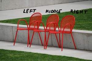
Okay, let's throw a (small) wrench into our work. How many ways can 4 people fill 3 chairs?

Answer

Again, for the sake of concreteness, let's name the four people Tom, Rick, Harry, and Mary and the chairs Left, Middle, and Right. If we fill the Left chair first, there are 4 possible people (Tom, Rick, Harry, and Mary). Let's suppose Tom is selected for the Left chair. Then, since Tom can't sit in more than one chair at a time when we fill the Middle chair, there are only 3 possible people (Rick, Harry, and Mary). If Rick is selected for the Middle chair, when we fill the Right chair, there are only 2 possible people (Harry and Mary). Putting all of this together, the Multiplication Principle tells us that there are:

$4\times 3\times 2$

or 24 possible ways to fill the three chairs.

Okay, okay! The main distinction between this example and the first example on this page is that the first example involves arranging all 4 people, whereas this example involves leaving one person out and arranging just 3 of the 4 people. This example allows us to introduce another generalization of the Multiplication Principle, namely the counting of the number of permutations of $n$ objects taken $r$ at a time, where $r\le n$.

Another Generalization of the Multiplication Principle

Suppose there are $r$ positions to be filled with $n$ different objects, in which there are:

$n$ choices for the 1st position
$n-1$ choices for the 2nd position
$n-2$ choices for the 3rd position
... and ...
$n-(r-1)$ choices for the last position

The Multiplication Principle tells us there are in general:

$n\times (n-1)\times (n-2)\times \ldots \times [n-(r-1)]$

ways of filling the $r$ positions. We can easily show that, in general, this quantity equals:

$\dfrac{n!}{(n-r)!}$

Here's how it works:

And, formally:

Permutation of $n$ objects taken $r$ at a time: ordered arrangement of $n$ different objects in $r$ positions. The number of such permutations is:
$_nP_r=\dfrac{n!}{(n-r)!}$

The subscripted $n$ represents the number of objects you are wanting to arrange, while the subscripted $r$ represents the number of positions you have for the objects to fill.

Example 3-9

An artist has 9 paintings. How many ways can he hang 4 paintings side-by-side on a gallery wall?

3.3 - Combinations

Example 3-10

Maria has three tickets for a concert. She'd like to use one of the tickets herself. She could then offer the other two tickets to any of four friends (Ann, Beth, Chris, Dave). How many ways can 2 people be selected from 4 to go to a concert?

Hmmm... could we solve this problem without creating a list of all of the possible outcomes? That is, is there a formula that we could just pull out of our toolbox when faced with this type of problem? Well, we want to find $C$, the number of unordered subsets of size $r$ that can be selected from a set of $n$ different objects.

We can determine a general formula for $C$ by noting that there are two ways of finding the number of ordered subsets (note that that says ordered, not unordered):

Method #1
We learned how to count the number of ordered subsets on the last page. It is just $_nP_r$, the number of permutations of $n$ objects taken $r$ at a time.
Method #2
Alternatively, we could take each of the $C$ unordered subsets of size $r$ and permute each of them to get the number of ordered subsets. Because each of the subsets contains $r$ objects, there are $r!$ ways of permuting them. Applying the Multiplication Principle then, there must be $C\times r!$ ordered subsets of size $r$ taken from $n$ objects.

Because we've just used two different methods to find the same thing, they better equal each other. That is, it must be true that:

$_nP_r=C\times r!$

Ahhh, we now have an equation that involves $C$, the quantity for which we are trying to find a formula. It's straightforward algebra at this point. Let's take a look.

Here's a formal definition.

combination of $n$ objects taken $r$ at a time

number of unordered subsets is:

$_nC_r=\dbinom{n}{r}=\dfrac{n!}{r!(n-r)!}$

We say “$n$ choose $r$.”

The $r$ represents the number of objects you'd like to select (without replacement and without regard to order) from the $n$ objects you have.

Example 3-11

Twelve (12) patients are available for use in a research study. Only seven (7) should be assigned to receive the study treatment. How many different subsets of seven patients can be selected?

Answer

The formula for the number of combinations of 12 objects taken 7 at a time tells us that there are:

$\dbinom{12}{7}=\dfrac{12!}{7!(12-7)!}=792$

different possible subsets of 7 patients that can be selected.

Example 3-12

Let's use a standard deck of cards containing 13 face values (Ace, 2, 3, 4, 5, 6, 7, 8, 9, 10, Jack, Queen, and King) and 4 different suits (Clubs, Diamonds, Hearts, and Spades) to play five-card poker. If you are dealt five cards, what is the probability of getting a "full-house" hand containing three kings and two aces (KKKAA)?

If you are dealt five cards, what is the probability of getting any full-house hand?

An Aside on Binomial Coefficients

The numbers:

$\dbinom{n}{r}$

are frequently called binomial coefficients, because they arise in the expansion of a binomial. Let's recall the expansion of $(a+b)^2$ and $(a+b)^3$.

Now, you might recall that, in general, the binomial expansion of $(a+b)^n$ is:

$(a+b)^n=\sum\limits_{r=0}^n \dbinom{n}{r} b^r a^{n-r}$

Let's see if we can convince ourselves as to why this is true.

Now, you might want to entertain yourself by verifying that the formula given for the binomial expansion does indeed work for $n=2$ and $n=3$.

3.4 - Distinguishable Permutations

Example 3-13

Suppose we toss a gold dollar coin 8 times. What is the probability that the sequence of 8 tosses yields 3 heads (H) and 5 tails (T)?

Answer

Two such sequences, for example, might look like this:

H H H T T T T T or this H T H T H T T T

Assuming the coin is fair, and thus that the outcomes of tossing either a head or tail are equally likely, we can use the classical approach to assigning the probability. The Multiplication Principle tells us that there are:

$2\times 2\times 2\times 2\times 2\times 2\times 2\times 2$

or 256 possible outcomes in the sample space of 8 tosses. (Can you imagine enumerating all 256 possible outcomes?) Now, when counting the number of sequences of 3 heads and 5 tosses, we need to recognize that we are dealing with arrangements or permutations of the letters, since order matters, but in this case not all of the objects are distinct. We can think of choosing (note that choice of word!) $r=3$ positions for the heads (H) out of the $n=8$ possible tosses. That would, of course, leave then $n-r=8-3=5$ positions for the tails (T). Using the formula for a combination of $n$ objects taken $r$ at a time, there are therefore:

$\dbinom{8}{3}=\dfrac{8!}{3!5!}=56$

distinguishable permutations of 3 heads (H) and 5 tails (T). The probability of tossing 3 heads (H) and 5 tails (T) is thus $\dfrac{56}{256}=0.22$.

Let's formalize our work here!

Distinguishable permutations of $n$ objects

Given $n$ objects with:

$r$ of one type, and
$n-r$ of another type

there are:

$_nC_r=\binom{n}{r}=\dfrac{n!}{r!(n-r)!}$

Let's take a look at another example that involves counting distinguishable permutations of objects of two types.

Example 3-14

the word Mississippi on the side of a building

How many ordered arrangements are there of the letters in MISSISSIPPI?

Answer

Well, there are 11 letters in total:

1 M, 4 I, 4 S and 2 P

We are again dealing with arranging objects that are not all distinguishable. We couldn't distinguish among the 4 I's in any one arrangement, for example. In this case, however, we don't have just two, but rather four, different types of objects. In trying to solve this problem, let's see if we can come up with some kind of a general formula for the number of distinguishable permutations of n objects when there are more than two different types of objects.

Let's formalize our work.

number of distinguishable permutations of $n$ objects

$n_1$ are of one type
$n_2$ are of a second type
... and ...
$n_k$ are of the last type

and $n=n_1+n_2+\ldots +n_k$is given by:

$\dbinom{n}{n_1n_2n_3\ldots n_k}=\dfrac{n!}{n_1!n_2!n_3! \ldots n_k!}$

Let's take a look at a few more examples involving distinguishable permutations of objects of more than two types.

Example 3-15

How many ordered arrangements are there of the letters in the word PHILIPPINES?

Answer

The number of ordered arrangements of the letters in the word PHILIPPINES is:

$\dfrac{11!}{3!1!3!1!1!1!1!}=1,108,800$

Example 3-16

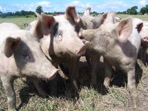
Fifteen (15) pigs are available to use in a study to compare three (3) different diets. Each of the diets (let's say, A, B, C) is to be used on five randomly selected pigs. In how many ways can the diets be assigned to the pigs?

Answer

Well, one possible assignment of the diets to the pigs would be for the first five pigs to be placed on diet A, the second five pigs to be placed on diet B, and the last 5 pigs to be placed on diet C. That is:

A A A A A B B B B B C C C C C

Another possible assignment might look like this:

A B C A B C A B C A B C A B C

Upon studying these possible assignments, we see that we need to count the number of distinguishable permutations of 15 objects of which 5 are of type A, 5 are of type B, and 5 are of type C. Using the formula, we see that there are:

$\dfrac{15!}{5!5!5!}=756756$

ways in which 15 pigs can be assigned to the 3 diets. That's a lot of ways!

3.5 - More Examples

We've learned a number of different counting techniques in this lesson. Now, we'll get some practice using the various techniques. As we do so, you might want to keep these helpful (summary) hints in mind:

When you begin to solve a counting problem, it's always, always, always a good idea to create a specific example (or two or three...) of the things you are trying to count.
If there are $m$ ways of doing one thing, and $n$ ways of doing another thing, then the Multiplication Principle tells us there are $m\times n$ ways of doing both things.
If you want to place $n$ things in $n$ positions, and you care about order, you can do it in $n!$ ways. (Doing so is called permuting $n$ items $n$ at a time.)
If you want to place $n$ things in $r$ positions, and you care about order, you can do it in $\dfrac{n!}{(n-r)!}$ ways. (Doing so is called permuting $n$ items $r$ at a time.)
If you have $m$ items of one kind, $n$ items of another kind, and $o$ items of a third kind, then there are $\dfrac{(m+n+o)!}{m!n!o!}$ ways of arranging the items. (Doing so is called counting the number of distinguishable permutations.)
If you have $m$ items of one kind and $n-m$ items of another kind, then there are $\dfrac{n!}{m!(n-m)!}$ ways of choosing the $m$ items without replacement and without regard to order. (Doing so is called counting the number of combinations, and we say "$n$ choose $m$".)

Let's take a look at some examples now!

Example 3-17

flags A ship's captain sends signals by arranging 4 orange and 3 blue flags on a vertical pole. How many different signals could the ship's captain possibly send?

Answer

If the flags were numbered 1, 2, 3, 4, 5, 6 and 7, then the orange flags and blue flags would be distinguishable among themselves. In that case, the ship's captain could send any of 7! = 5,040 possible signals.

The flags are not numbered, however. That is, the four orange flags are not distinguishable among themselves, and the 3 blue flags are not distinguishable among themselves. We need to count the number of distinguishable permutations when the two colors are the only features that make the flags distinguishable. The ship's captain has 4 orange flags and 3 blue flags. Using the formula for the number of distinguishable permutations, the ship's captain could send any of:

$\dfrac{7!}{4!3!}=\dbinom{7}{4}$

or 35 possible signals.

By the way, recall that the 4! in the denominator reduces the number of 7! arrangements by the number of ways in which the four orange flags could have been arranged had they been distinguishable among themselves (if they were labeled 1, 2, 3, 4, for example). Likewise, the 3! in the denominator reduces the number of 7! arrangements by the number of ways in which the three blue flags could have been arranged had they been distinguishable among themselves (if they were labeled 1, 2, 3, for example).

Example 3-18

Now the ship's captain sends signals by arranging 3 red, 4 orange and 2 blue flags on a vertical pole. How many different flags signals could the ship's captain possibly send?

Answer

Again, if the flags were numbered 1, 2, 3, 4, 5, 6, 7, 8, and 9, then the red, yellow, and blue flags would be distinguishable among themselves. In that case, the ship's captain could send any of $9!=362,880$ possible signals.

The flags are not numbered, however. That is, the three red flags are not distinguishable among themselves, the four orange flags are not distinguishable among themselves, and the 2 blue flags are not distinguishable among themselves. We need to count the number of distinguishable permutations when the three colors are the only features that make the flags distinguishable. Again, using the formula for the number of distinguishable permutations, the ship's captain could send any of:

$\dfrac{9!}{4!3!2!}=\dbinom{9}{4\ 3\ 2}$

or 1260 possible signals.

Example 3-19

How many four-letter codes are possible?

Answer

One example of a four-letter code is XSST. Another example is RLPR. If we were to try to enumerate all of the possible four-letter codes, we'd have to place any of 26 letters in the first position, any of 26 letters in the second position, any of 26 letters in the third position, and any of 26 letters in the fourth position:

___ , ___ , ___ , ___

Yikes, that sounds like a lot of work! Fortunately, the Multiplication Principle tells us to simply multiply those 26's together. That is, there are:

$26 \times 26 \times 26\times 26=456,976$

possible four-letter codes.

Now, let's add a restriction. How many four-letter codes are possible if no letter may be repeated?

Answer

One example of a four-letter code, with no letters repeated, is XSGT. Another such example is RLPW. If we were to try to enumerate all of the possible four-letter codes with no letters repeated, we'd have to place any of 26 letters in the first position. Then, since one of the letters would be chosen for the first position, we'd have to place any of 25 letters in the second position. Then, since two of the letters would be chosen for the first and second positions, we'd have to place any of 24 letters in the third position. Finally, since three of the letters would be chosen for the first, second, and third positions, we'd have to place any of 23 letters in the fourth position:

___ , ___ , ___ , ___

Again, the Multiplication Principle tells us to simply multiply the numbers together. When we don't allow repetition of letters, there are:

$26\times 25\times 24\times 23=358, 800$

possible four-letter codes. By the way, we could alternatively recognize here that we are permuting 26 letters, 4 at a time, and then use the formula for a permutation of 26 objects (letters) taken 4 at a time:

$_{26}P_4=\dfrac{26!}{22!}=26\times 25 \times 24 \times 23$

Either way, we still end up counting 358,800 possible four-letter codes.

Now, let's add yet another restriction. How many four-letter codes are possible if no repetition is allowed and order is not important?

Answer

Again, one example of a four-letter code, with no letters repeated, is XSGT. In this case, however, we would not distinguish the code XSGT from the code TGSX. That is, all we care about is counting how many ways we can choose any four letters from the 26 possible letters in the alphabet. So, we sample without replacement (to ensure no letters are repeated) and we don't care about the order in which the letters are chosen. It sounds like the formula for a combination will do the trick then. It tells us that there are:

$_{26}C_4=\dfrac{26!}{22!4!}$

or 14,950 four-letter codes when order doesn't matter and repetition is not permitted.

By the way, the formula here differs from the formula in the previous example by having a $4!$ in the denominator. The $4!$ appears in the denominator because we added the restriction that the order of the letters doesn't matter. Therefore, we want to divide by the number of ways we over-counted, that is, by the $4!$ ways of ordering the four letters. That is, the $4!$ in the denominator reduces the number of $\dfrac{26!}{22!}$ arrangements counted in the previous example by the number of ways in which the four letters could have been ordered.

If you hadn't noticed already, you might want to take note now that the solutions to each of the three previous examples started out by highlighting a specific example (or two) of the kinds of four-letter codes we were trying to count. This is a really good practice to follow when trying to count objects. After all, it is awfully hard to count correctly if you don't know what it is you are counting!

Example 3-20

In how many ways can 4 heterosexual married couples (1 male, 1 female) attending a concert be seated in a row of 8 seats if there are no restrictions as to where the 8 can sit?

Answer

Here are the eight seats:

seats

If we arbitrarily name the people A, B, C, D, E, F, G, and H, then one possible seating arrangement is ABCDEFGH. Another is DGHCAEBF. These examples suggest that we have to place 8 people into 8 seats without repetition. That is, one person can't occupy two seats!

Well, we can place any of the 8 people in the first seat. Then, since one of the people would be chosen for the first seat, we'd have to place any of the remaining 7 people in the second seat. Then, since two of the people would be chosen for the first and second seats, we'd have to place any of the remaining 6 people in the third seat. And so on ... until we have just one person remaining to occupy the last seat. The Multiplication Principle tells us to multiply the numbers together. That is, there are:

$8\times 7\times 6\times 5\times 4\times 3\times 2\times 1=40, 320$

possible seating arrangements. Of course, we alternatively could have recognized that we are trying to count the number of permutations of 8 objects taken 8 at a time. The permutation formula would tell us similarly that there are $8! = 40,320$ possible seating arrangements.

Now, let's add a restriction. In how many ways can 4 married couples attending a concert be seated in a row of 8 seats if each married couple is seated together?

Answer

Here are the eight seats shown as four paired seats:

seats

If we arbitrarily name the people A1, A2, B1, B2, C1, C2, D1, and D2, then one possible seating arrangement is B2, B1, A1, A2, C2, C1, D1, D2. Another such assignment might be B1, B2, A2, A1, C1, C2, D1, D2. These two examples illustrate that counting here is a two-step process. First, we have to figure out how many ways the couples A, B, C, and D can be arranged. Permuting 4 items (couples) 4 at a time... there are 4! ways. Then, we have to arrange the partners within each couple. Well, couple A can be arranged 2! ways. We can even list the ways... they can sit either as A1, A2 or as A2, A1. Likewise, couple B can be arranged in 2! ways, as can couples C and D. The Multiplication Principle then tells us to multiply all the numbers together. Four married couples can be seated in a row of 8 seats in:

$4!\times 2!\times 2!\times 2!\times 2!=384$ ways

if each married couple is seated together.

Are you enjoying this?! Now, let's add a different restriction. In how many ways can 4 married couples attending a concert be seated in a row of 8 seats if members of the same sex are all seated next to each other?

Answer

Here are the eight seats, shown as two sets of fours seats:

seats

If we arbitrarily name the people M1, M2, M3, M4 and F1, F2, F3, F4, then one possible seating arrangement is M1, M2, M4, M3, F2, F1, F3, F4. Another such assignment might be F1, F2, F4, F3, M2, M1, M4, M3. Again, these two examples illustrate that counting here is a two-step process. First, we have to figure out how many ways the genders M and F can be arranged. There are, of course, 2 ways... the males in the seats on the left and females in the seats on the right or the females in the seats on the left and the males in the seats on the right. Then, we have to arrange the people within each gender. Let's take the females first. Permuting 4 items (females) 4 at a time... there are $4!$ ways. Likewise, there are $4!$ ways of arranging the males within their 4 seats. The Multiplication Principle then tells us to multiply all the numbers together. Four married couples can be seated in a row of 8 seats in:

$4!\times 4!\times 2=1,152$ ways

if the members of the same sex are seated next to each other.

You might want to note again that the solutions to each of the three previous examples started out by highlighting a specific example (or two) of the kinds of seating arrangements we were trying to count. Doing so really does help get you started in the right direction!

Example 3-21

How many ways are there to choose non-negative integers $a, b, c, d, \text{ and }e$, such that the non-negative integers add up to 6, that is:

$a+b+c+d+e=6$

Answer

This is definitely a counting problem where you'll want to start by looking at a few examples first! One such example is:

$1+2+1+0+2=6$

where $a = 1,\; b = 2,\; c = 1,\; d = 0,\text{ and }e = 3$. Another example is:

$1+0+1+4+0=6$

where $a = 1,\; b = 0,\; c = 1,\; d = 4,\text{ and }e = 0$. And one last example is:

$0 + 0 + 0 + 0 + 6 = 6$

where $a = 0,\; b = 0,\; c = 0, \;d = 0,\text{ and }e = 6$. So, what have we learned from these examples? Well, one thing becomes clear, if it wasn't already, is that $a, b, c, d,\text{ and }e$ must each be an integer between 0 and 6.

Now, to advance our solution, we'll use what is called the "stars-and-bars" method. Because the sum that we are trying to obtain is 6, we'll divvy 6 stars into 5 bins called $a, b, c, d, \text{ and }e$. If we arrange the 6 stars in a row, we can use 4 bars to represent the bins' walls. Here's what the stars-and-bars would look like for our first example in which $1 + 2 + 1 + 0 + 2 = 6$:

The first bin, $a$, has 1 star; the second bin, $b$, has 2 stars; the third bin, $c$, has 1 star; the fourth bin, $d$, has 0 stars; and the fifth bin, $e$, has 2 stars. Now, here's what the stars-and-bars would look like for our second example in which $1 + 0 + 1 + 4 + 0 = 6$:

Notice that two bars adjacent either to each other or a bar at the end of the row of the stars implies that that bin has 0 stars in it. Here's what the stars-and-bars would look like for our last example in which $0 + 0 + 0 + 0 + 6 = 6$:

Here, the first bin, $a$, has 0 stars; the second bin, $b$, has 0 stars; the third bin, $c$, has 0 stars; the fourth bin, $d$, has 0 stars; and the fifth bin, $e$, has 6 stars. All we've done so far is look at examples! By doing so though, perhaps we are now ready to make the jump to see that enumerating all of the possible ways of getting 5 non-negative integers to sum to 6 reduces to counting the number of distinguishable permutations of 10 items... of which 4 items are bars and 6 items are stars. That is, there are:

$\dfrac{10!}{6!4!}=210$ ways

to choose non-negative integers $a, b, c, d, \text{ and }e$, such that the non-negative integers add up to 6.

Do you get it? Try this next one out to test yourself. How many ways are there to choose non-negative integers $a$ and $b$such that the non-negative integers add up to 5, that is:

$a + b = 5$

One such example is $1 + 4 = 5$. Its stars-and-bars graphic would look like this:

The stars-and-bars graphic for $2 + 3 = 5$ would look like this:

In this case, we have to count the number of distinguishable permutations of 6 items... of which 1 item is a bar and 5 items are stars. There are thus:

$\dfrac{6!}{5!1!}=6$ ways

to choose non-negative integers $a$ and $b$ such that the non-negative integers add up to 5.

Are you ready for another one? How many ways can you specify 89 non-negative integers such that the non-negative integers add up to 258? Do you see a pattern from the previous examples? If we are trying to obtain a sum of some number $m$ using $k+1$ non-negative integers, then the stars-and-bars method tells us we'd need to count the number of permutations of $m$ stars and $k$ bars. In general, then, there are:

$\dfrac{(m+k)!}{m!k!}$

ways of obtaining the sum $m$ using $k+1$ non-negative integers.

Lesson 4: Conditional Probability

Overview

In this lesson, we'll focus on finding a particular kind of probability called a conditional probability. In short, a conditional probability is a probability of an event given that another event has occurred. For example, rather than being interested in knowing the probability that a randomly selected male has prostate cancer, we might instead be interested in knowing the probability that a randomly selected male has prostate cancer given that the male has an elevated prostate-specific antigen. We'll explore several such conditional probabilities.

Objectives

Upon completion of this lesson, you should be able to:

Understand the definition of conditional probability.
Learn how to use the relative frequency approach to assigning probability to find the conditional probability of an event from a two-way table.
Learn how to use the formula for conditional probability.
Learn how to use the multiplication rule to find the probability of the intersection of two events.
Learn how to use the multiplication rule to find the probability of the intersection of more than two events.
Learn to apply the techniques learned in the lesson to new problems.

4.1 - The Motivation

Example 4-1

A researcher is interested in evaluating how well a diagnostic test works for detecting renal disease in patients with high blood pressure. She performs the diagnostic test on 137 patients — 67 with known renal disease and 70 who are known to be healthy. The diagnostic test comes back either positive (the patient has renal disease) or negative (the patient does not have renal disease). Here are the results of her experiment:

	Test Results
Truth	Positive	Negative	Total
Renal Disease	44	23	67
Healthy	10	60	70
Total	54	83	137

If we let $T+$ be the event that the person tests positive, we can use the relative frequency approach to assigning probability to determine that:

$P(T+)=\dfrac{54}{137}$

because, of the 137 patients, 54 tested positive. If we let $D$ be the event that the person is truly diseased, we determine that:

$P(D)=\dfrac{67}{137}$

because, of the 137 patients, 67 are truly diseased. That's all well and good, but the question that the researcher is really interested in is this:

If a person has renal disease, what is the probability that he/she tests positive for the disease?

The blue portion of the question is a "conditional", while the green portion is a "probability." Aha... do you get it? These are the kinds of questions that we are going to be interested in answering in this lecture, and hence its title "Conditional Probability." Now, let's just push this example a little bit further, and in so doing introduce the notation we are going to use to denote a conditional probability.

We can again use the relative frequency approach and the data the researcher collected to determine:

$P(T+|D)=\dfrac{44}{67}=0.65$

That is, the probability a person tests positive given he/she has renal disease is 0.65. There are a couple of things to note here.

First, the notation $P(T+|D)$ is standard conditional probability notation. It is read as "the probability a person tests positive given he/she has renal disease." The bar ( | ) is always read as "given." The probability we are looking for precedes the bar, and the conditional follows the bar.

Second, note that determining the conditional probability involves a two-step process. In the first step, we restrict the sample space to only those (67) who are diseased. Then, in the second step, we determine the number of interest (44) based on the new sample space.

Hmmm.... rather than having to do all of this thinking (!), can't we just derive some sort of general formula for finding a conditional probability?

In the next section, we generalize our derived formula.

4.2 - What is Conditional Probability?

Conditional Probability

The conditional probability of an event $A$ given that an event $B$ has occurred is written:

$P(A|B)$

and is calculated using:

$P(A|B)=\dfrac{P(A\cap B)}{P(B)}$

as long as $P(B)>0$.

Example 4-1 Continued

Let's return to our diagnostic test for renal disease. Recall that the researcher collected the following data:

Test Results
Truth	Positive	Negative	Total
Renal Disease	44	23	67
Healthy	10	60	70
Total	54	83	137

Now, when a researcher is developing a diagnostic test, the question she cares about is the one we investigated previously, namely:

If a person has renal disease, what is the probability of testing positive?

This quantity is what we would call the "sensitivity" of a diagnostic test. As patients, we are interested in knowing what is called the "positive predictive value" of a diagnostic test. That is, we are interested in this question:

If I receive a positive test, what is the probability that I actually have the disease?

We would hope, of course, that the probability is 1. But, only rarely is a diagnostic test perfect. The collected data suggest that the renal disease test is not perfect. How good is it? That is, what is the positive predictive value of the test?

Properties of Conditional Probability

Because conditional probability is just a probability, it satisfies the three axioms of probability. That is, as long as $P(B)>0$:

$P(A|B)\ge0$
$P(B|B)=1$
If $A_1, A_2, \ldots, A_k$ are mutually exclusive events, then $P(A_1\cup A_2\cup \ldots \cup A_k|B)=P(A_1|B)+P(A_2|B)+\ldots+P(A_k|B)$ and likewise for infinite unions.

The "proofs" of the first two axioms are straightforward:

The "proof" of the third axiom is also straightforward. It just takes a little more work:

Example 4-3

A box contains 6 white balls and 4 red balls. We randomly (and without replacement) draw two balls from the box. What is the probability that the second ball selected is red, given that the first ball selected is white?

What is the probability that both balls selected are red?

The second method used in solving this problem used what is known as the multiplication rule. Now that we've actually used the rule, let's now go and generalize it!

4.3 - Multiplication Rule

Multiplication Rule

The probability that two events A and B both occur is given by:

$P(A\cap B)=P(A|B)P(B)$

or by:

$P(A\cap B)=P(B|A)P(A)$

Example 4-4

A box contains 6 white balls and 4 red balls. We randomly (and without replacement) draw two balls from the box. What is the probability that the second ball selected is red?

We'll see calculations like the one just made over and over again when we study Bayes' Rule.

The Multiplication Rule Extended

The multiplication rule can be extended to three or more events. In the case of three events, the rule looks like this:

$P(A \cap B \cap C)=P[(A \cap B) \cap C)]=\underbrace{P(C | A \cap B)}_{a} \times \underbrace{P(A \cap B)}_{b}$

$\text { But since } P(A \cap B)=\underbrace{P(B | A) \times P(A)}_{b}\colon$

$P(A \cap B \cap C)=\underbrace{P(C | A \cap B)}_{a} \times \underbrace{P(B | A) \times P(A)}_{b}$

Example 4-5

Three cards are dealt successively at random and without replacement from a standard deck of 52 playing cards. What is the probability of receiving, in order, a king, a queen, and a jack?

4.4 - More Examples

Example 4-6

A drawer contains:

4 red socks
6 brown socks
8 green socks

A man is getting dressed one morning and barely awake when he randomly selects 2 socks from the drawer (without replacement, of course). What is the probability that both of the socks he selects are green given that they are the same color? If we define four events as such:

Let $R_i$ = the event the man selects a red sock on selection $i$ for $i = 1, 2$
Let $B_i$ = the event the man selects a brown sock on selection $i$ for $i = 1, 2$
Let $G_i$ = the event the man selects a green sock on selection $i$ for $i = 1, 2$
Let $S$ = the event that the 2 socks selected are the same color

then we are looking for the following conditional probability:

$P(G_1\text{ and }G_2|S)$

Let's give it a go.

Example 4-7

Medical records reveal that of the 937 men who died in a particular region in 1999:

212 of the men died of causes related to heart disease,
312 of the men had at least one parent with heart disease

Of the 312 men with at least one parent with heart disease, 102 died of causes related to heart disease. Using this information, if we randomly select a man from the region, what is the probability that he dies of causes related to heart disease given that neither of his parents died from heart disease? If we define two events as such:

Let $H$ = the event that at least one of the parents of a randomly selected man died of causes related to heart disease
Let $D$= the event that a randomly selected man died of causes related to heart disease

then we are looking for the following conditional probability:

$P(D|H^\prime)$

The following viewlet uses a Venn diagram to help us work through this problem. Just click on the Inspect! icon when you're good and ready (you'll no doubt want to use the pause and play buttons freely):

If a Venn diagram doesn't do it for you, perhaps an alternative way will:

Lesson 5: Independent Events

Overview

In this lesson, we learn what it means for two (or more) events to be independent. We'll formally learn, for example, why we say that the outcome of the flip of a fair coin is independent of the flips that came before it.

Objectives

Upon completion of this lesson, you should be able to:

Learn how to determine if two events are independent.
Learn how to find the probability of the intersection of two events if the two events are independent.
Learn how to determine if three or more events are pairwise independent.
Learn how to determine if three or more events are mutually independent.
Understand each step of the proofs contained in the lesson.
Practice applying the techniques learned in the lesson to new problems.

5.1 - Two Definitions

Example 5-1

A couple plans to have three children. What is the probability that the second child is a girl? And, what is the probability that the second child is a girl given that the first child is a girl?

This example leads us to a formal definition of independent events.

Independent Events: Events $A$ and $B$ are independent events if the occurrence of one of them does not affect the probability of the occurrence of the other. That is, two events are independent if either:

$P(B|A)=P(B)$

(provided that $P(A)>0$) or:

$P(A|B=P(A))$

(provided that $P(B)>0$).

Now, since independence tells us that $P(B|A)=P(B)$, we can substitute $P(B)$ in for $P(B|A)$ in the formula given to us by the multiplication rule:

$P(A\cap B)=P(A)\times P(B|A)$

yielding:

$P(A\cap B)=P(A)\times P(B)$

This substitution leads us to an alternative definition of independence.

Independent Events

Events $A$ and $B$ are independent events if and only if :

$P(A\cap B)=P(A)\times P(B)$

Otherwise, $A$ and $B$ are called dependent events.

Recall that the "if and only if" (often written as "iff") in that definition means that the if-then statement works in both directions. That is, the definition tells us two things:

If events $A$ and $B$ are independent, then $P(A\cap B)=P(A)\times P(B)$.
If $P(A\cap B)=P(A)\times P(B)$, then events $A$ and $B$ are independent.

The next example illustrates the first of these two directions, while the second example illustrates the second direction.

Example 5-2

A recent survey of students suggested that 10% of Penn State students commute by bike, while 40% of them have a significant other. Based on this survey, what percentage of Penn State students commute by bike and have a significant other?

Answer

Let's let $B$ be the event that a randomly selected Penn State student commutes by bike and $S$ be the event that a randomly selected Penn State student has a significant other. If $B$ and $S$ are independent events (okay??), then the definition tells us that:

$P(B\cap S)=P(B)\times P(S)=0.10(0.40)=0.04$

That is, 4% of Penn State students commute by bike and have a significant other. (Is this result at all meaningful??)

Example 5-3

Let's return to the couple that plans to have three children. Is the event that the couple's third child is a girl independent of the event that the couple's first two children are girls?

Answer

Again, letting $G$ denote girl and $B$ denote boy, the sample space of the genders of the couple's three children looks like this:

$\{GGG, GGB, GBG, BGG, BBG, BGB, GBB, BBB\}$

Let $C$ be the event that the couple's first two children are girls, and let $D$ be the event that the third child is a girl. Then event $C$ looks like this:

$\{GGG, GGB\}$

where the first two children are restricted to be girls ($G$), while the third child could be either a girl ($G$) or a boy ($B$). For event $D$, there are no restrictions on the first two children, but the third child must be a girl. Therefore, event $D$ looks like this:

$\{GGG, BBG, BGG, GBG\}$

Now, $C\cap D$ is the event that all three children are girls and hence it looks like:

$\{GGG\}$

Using the classical approach to assigning a probability to the three events $C, D$ and $C\cap D$:

$P(C) = \dfrac{2}{8}$
$P(D) = \dfrac{4}{8}$
$P(C\cap D) = \dfrac{1}{8}$

Now, since:

$P(C)\times P(D)=\dfrac{2}{8}\left(\dfrac{4}{8}\right)=\dfrac{8}{64}=\dfrac{1}{8}=P(C\cap D)$

we can conclude that events $C$ and $D$ are independent. That is, the event that the couple's third child is a girl is independent of the event that the first two children were girls. This result seems quite intuitive, eh? If so, then it is quite interesting that so many people fall prey to the "Gambler's Fallacy" illustrated in the next example.

Example 5-4

A man tosses a fair coin eight times and observes whether the toss yields a head (H) or a tail (T) on each toss. Which of the following sequences of coin tosses is the man more likely to get a head (H) on his next toss? This one:

$ TTTTTTTT$

or this one:

$HHTHTTHH$

The answer is neither as illustrated here:

The moral of the story is to be careful not to fall prey to "Gambler's Fallacy," which occurs when a person mistakenly assumes that a departure from what occurs on average in the long term will be corrected in the short term. In this case, a person would be mistaken to think that just because the coin was departing from the average (half the tosses being heads and half the tosses being tails) by getting eight straight tails in row that a head was due to be tossed. A classic example of Gambler's Fallacy occurred on August 18, 1913 at the casino in Monte Carlo, in which:

... black came up a record twenty-six times in succession [in roulette]. … [There] was a near-panicky rush to bet on red, beginning about the time black had come up a phenomenal fifteen times. In application of the maturity [of the chances] doctrine, players doubled and tripled their stakes, this doctrine leading them to believe after black came up the twentieth time that there was not a chance in a million of another repeat. In the end the unusual run enriched the Casino by some millions of francs. [Source: Darrell Huff & Irving Geis, How to Take a Chance (1959), pp. 28-29.]

A joke told among statisticians demonstrates the nature of the fallacy. A man attempts to board an airplane with a bomb. When questioned by security, he explains that he was just trying to protect himself: "The chances of an airplane having a bomb on it are very small," he reasons, "and certainly the chances of having two are almost none!" A similar example is in the book by John Irving called The World According to Garp, in which the hero Garp decides to buy a house immediately after a small plane crashes into it, reasoning that the chances of another plane hitting the house have just dropped to zero.

5.2 - Three Theorems

On this page, we present, prove, and then use three sometimes helpful theorems.

Theorem: If $A$ and $B$ are independent events, then the events $A$ and $B^\prime$ are also independent

Theorem: If $A$ and $B$ are independent events, then the events $A^\prime$ and $B$ are also independent

Theorem: If $A$ and $B$ are independent events, then the events $A^\prime$ and $B^\prime$ are also independent.

Example 5-5

A nationwide poll determines that 72% of the American population loves eating pizza. If two people are randomly selected from the population, what is the probability that the first person loves eating pizza, while the second one does not?

Answer

Let $A$ be the event that the first person loves pizza, and let $B$ be the event that the second person loves pizza. Because the two people are selected randomly from the population, it is reasonable to assume that $A$ and $B$ are independent events. If $A$ and $B$ are independent events, then $A$ and $B^\prime$ are also independent events. Therefore, $P(A\cap B^\prime)$, the probability that the first person loves eating pizza, while the second one does not can be calculated by multiplying their individual probabilities together. That is, the probability that the first person loves eating pizza, while the second one does not is:

$P(A\cap B^\prime)=0.72(1-0.72)=0.202$

5.3 - Mutual Independence

Example 5-6

Consider a roulette wheel that has 36 numbers colored red ($R$) or black ($B$) according to the following pattern:

1	2	3	4	5	6	7	8	9	10	11	12	13	14	15	16	17	18
R	R	R	R	R	B	B	B	B	R	R	R	R	B	B	B	B	B
36	35	34	33	32	31	30	29	28	27	26	25	24	23	22	21	20	19

and define the following three events:

Let $A$ be the event that a spin of the wheel yields a RED number = $\{1, 2, 3, 4, 5, 10, 11, 12, 13, 24, 25, 26, 27, 32, 33, 34, 35, 36\}$.
Let $B$ be the event that a spin of the wheel yields an EVEN number = $\{2, 4, 6, 8, 10, 12, 14, 16, 18, 20, 22, 24, 26, 28, 30, 32, 34, 36\}$.
Let $C$ be the event that a spin of the wheel yields a number no greater than 18 = $\{1, 2, 3, 4, 5, 6, 7, 8, 9, 10, 11, 12, 13, 14, 15, 16, 17, 18\}$.

Now consider the following two questions:

Are the events $A$, $B$, and $C$ "pairwise independent?" That is, is event $A$ independent of event $B$; event $A$ independent of event $C$; and $B$ independent of event $C$?
Does $P(A\cap B\cap C)=P(A)\times P(B)\times P(C)$?

Let's take a look:

So... this example illustrates that something seems to be lacking for the complete independence of events $A, B, \text{ and }C$. And, that's why the second condition exists in the following definition.

Mutually Independent Event

Three events $A, B,\text{ and }C$ are mutually independent if and only if the following two conditions hold:

The events are pairwise independent. That is,
- $P(A\cap B)=P(A)\times P(B)$ and...
- $P(A\cap C)=P(A)\times P(C)$ and...
- $P(B\cap C)=P(B)\times P(C)$
$P(A\cap B\cap C)=P(A)\times P(B)\times P(C)$

The idea of mutual independence can be extended to four or more events — each pair, triple, quartet, and so on, must satisfy the above type of multiplication rule.

Example 5-7

One ball is drawn randomly from a bowl containing four balls numbered 1, 2, 3, and 4. Define the following three events:

Let $A$ be the event that a 1 or 2 is drawn. That is, $A=\{1, 2\}$.
Let $B$ be the event that a 1 or 3 is drawn. That is, $B = \{1, 3\}$.
Let $C$ be the event that a 1 or 4 is drawn. That is, $C = \{1, 4\}$.

Are events $A, B,\text{ and }C$ pairwise independent? Are they mutually independent?

This example illustrates, as does the previous example, that pairwise independence among three events does not necessarily imply that the three events are mutually independent.

Example 5-8

A pair of fair six-sided dice is tossed once yielding the following sample space:

$S=\left\{\begin{array}{l}{(1,1)(1,2)(1,3)(1,4)(1,5)(1,6)} \\ {(2,1)(2,2)(2,3)(2,4)(2,5)(2,6)} \\ {(3,1)(3,2)(3,3)(3,4)(3,5)(3,6)} \\ {(4,1)(4,2)(4,3)(4,4)(4,5)(4,6)} \\ {(5,1)(5,2)(5,3)(5,4)(5,5)(5,6)} \\ {(6,1)(6,2)(6,3)(6,4)(6,5)(6,6)}\end{array}\right.$

Define the following three events:

Let $A$ be the event that the first die is a 1, 2, or 3.
Let $B$ be the event that the first die is a 3, 4, or 5.
Let $C$ be the event that the sum of the two faces equals 9. That is $C = \{(3,6), (6,3), (4,5), (5,4)\}$.

Are events $A, B,\text{ and }C$ pairwise independent? Are they mutually independent?

In solving that problem, I admit to being a little loosey-goosey with the definition of "mutual independence." That's why I said "a sort of mutual independence." Now that I haven't been perfectly clear so far, let me set the record straight by being perfectly clear. This example illustrates that the second condition of mutual independence among the three events $A, B,\text{ and }C$ (that is, the probability of the intersection of the three events equals the probabilities of the individual events multiplied together) does not necessarily imply that the first condition of mutual independence holds (that is, three events $A, B,\text{ and }C$ are pairwise independent). In order to check for mutual independence, you clearly need to check both the first and second conditions.

5.4 - A Closing Example

Example 5-9

A zealous father is trying to advance his son Jake's promising tennis career. Jake's father tells Jake that he'll give him \$500 if he wins (at least) two tennis sets in a row in a three-set series to be played with his father and the club champion alternately. The champion is a better player than Jake's father. Jake can choose who he plays first. If he plays his father first, he plays his father twice... first father, then champion, then father. If he plays the champion first, he plays his father once... first champion, then father, then champion. Which three-set series should Jake choose so as to maximize his chances of winning the \$500?

NOTE! This problem was adapted from problem #2 appearing in Fifty Challenging Problems in Probability, by Frederick Mosteller.

Solution

Because the champion plays better than the father, it seems reasonable that fewer sets should be played with the champion. On the other hand, the middle set is the key one, because Jake cannot get two wins in a row without winning the middle set. Now, let's define the following:

Let $C$stand for champion.
Let $F$ stand for father.
Let $W$ denote the event that Jake wins a set. Let $f$ denote the probability that Jake wins any set from his father. Let $c$ denote the probability that Jake wins any set from the champion.
Let $L$ denote the event that Jake loses a set.

Let's first consider the case where Jake plays in $F-C-F$ order (his father first, then the champion, then his father):

Now, let's consider the case where Jake plays in $C-F-C$ order (the champion first, then his father, then the champion):

In summary, the probability that Jake wins at least two sets in a row if he plays in $F-C-F$ order, is $fc(2-f)$, and the probability that Jake wins at least two sets in a row if he plays in $C-F-C$ order is $fc(2-c)$. For example, if $f=0.8$ and $c=0.4$, then the probability that Jake wins if he plays in $F-C-F$ order is 0.384, while the probability that Jake wins if he plays in $C-F-C$ order is 0.512. Now, because Jake is more likely to beat his father than to beat the champion, $f$ is larger than $c$, and $2-f$ is smaller than $2-c$. Therefore, in general, $fc(2-c)$ is larger than $fc(2-f)$. That is, Jake is more likely to win the \$500 if he plays the champion first, his father second, and the champion again. As such, it appears that the importance of winning the middle game outweighs the disadvantage of playing the champion twice!

Lesson 6: Bayes' Theorem

Overview

In this lesson, we'll learn about a classical theorem known as Bayes' Theorem. In short, we'll want to use Bayes' Theorem to find the conditional probability of an event $P(A|B)$, say, when the "reverse" conditional probability $P(B|A)$ is the probability that is known.

Objectives

Upon completion of this lesson, you should be able to:

Learn how to find the probability of an event by using a partition of the sample space $\mathbf{S}$.
Learn how to apply Bayes' Theorem to find the conditional probability of an event when the "reverse" conditional probability is the probability that is known.

6.1 - An Example

Example 6-1

A desk lamp produced by The Luminar Company was found to be defective ($D$). There are three factories ($A, B, C$) where such desk lamps are manufactured. A Quality Control Manager (QCM) is responsible for investigating the source of found defects. This is what the QCM knows about the company's desk lamp production and the possible source of defects:

Factory	% of total production	Probability of defective lamps
$A$	$0.35=P(A)$	$0.015=P(D\|A)$
$B$	$0.35=P(B)$	$0.010=P(D\|B)$
$C$	$0.30=P(C)$	$0.020=P(D\|C)$

The QCM would like to answer the following question: If a randomly selected lamp is defective, what is the probability that the lamp was manufactured in factory $C$?

Now, if a randomly selected lamp is defective, what is the probability that the lamp was manufactured in factory $A$? And, if a randomly selected lamp is defective, what is the probability that the lamp was manufactured in factory $B$?

Answer

In our previous work, we determined that $P(D)$, the probability that a lamp manufactured by The Luminar Company is defective, is 0.01475. In order to find $P(A|D)$ and $P(B|D)$ as we are asked to find here, we need to perform a similar calculation to the one we used in finding $P(C|D)$. Our work here will be simpler, though, since we've already done the hard work of finding $P(D)$. The probability that a lamp was manufactured in factory A given that it is defective is:

$P(A|D)=\dfrac{P(A\cap D)}{P(D)}=\dfrac{P(D|A)\times P(A)}{P(D)}=\dfrac{(0.015)(0.35)}{0.01475}=0.356$

And, the probability that a lamp was manufactured in factory $B$ given that it is defective is:

$P(B|D)=\dfrac{P(B\cap D)}{P(D)}=\dfrac{P(D|B)\times P(B)}{P(D)}=\dfrac{(0.01)(0.35)}{0.01475}=0.237$

Note that in each case we effectively turned what we knew upside down on its head to find out what we really wanted to know! We wanted to find $P(A|D)$, but we knew $P(D|A)$. We wanted to find $P(B|D)$, but we knew $P(D|B)$. We wanted to find $P(C|D)$, but we knew $P(D|C)$.It is for this reason that I like to say that we are interested in finding "reverse conditional probabilities" when we solve such problems.

The probabilities $P(A), P(B),\text{ and }P(C)$ are often referred to as prior probabilities, because they are the probabilities of events $A$, $B$, and $C$ that we know prior to obtaining any additional information. The conditional probabilities $P(A|D)$, $P(B|D)$, and $P(C|D)$ are often referred to as posterior probabilities, because they are the probabilities of the events after we have obtained additional information.

As a result of our work, we determined:

$P(C | D) = 0.407$
$P(B | D) = 0.237$
$P(A | D) = 0.356$

Calculated posterior probabilities should make intuitive sense, as they do here. For example, the probability that the randomly selected desk lamp was manufactured in Factory $C$ has increased, that is, $P(C|D)>P(C)$, because Factory $C$ generates the greatest proportion of defective lamps ($P(D|C)=0.02$). And, the probability that the randomly selected desk lamp was manufactured in Factory $B$ has decreased, that is, $P(B|D)<P(B)$, because Factory $B$ generates the smallest proportion of defective lamps ($P(D|B)=0.01$). It is, of course, always a good practice to make sure that your calculated answers make sense.

Let's now go and generalize the kind of calculation we made here in this defective lamp example .... in doing so, we summarize what is called Bayes' Theorem.

6.2 - A Generalization

Bayes' Theorem

Let the $m$ events $B_1, B_2, \ldots, B_m$ constitute a partition of the sample space $\mathbf{S}$. That is, the $B_i$ are mutually exclusive:

$B_i\cap B_j=\emptyset$ for $i\ne j$

and exhaustive:

$\mathbf{S}=B_1\cup B_2\cup \ldots B_m$

Also, suppose the prior probability of the event $B_i$is positive, that is, $P(B_i)>0$ for $i=1, \ldots, m$. Now, if $A$ is an event, then $A$ can be written as the union of $m$ mutually exclusive events, namely:

$A=(A\cap B_1)\cup(A\cap B_2)\cup\ldots\cup (A\cap B_m)$

Therefore:

\begin{align} P(A) &= P(A\cap B_1)+P(A\cap B_2)+\ldots +P(A\cap B_m)\\ &= \sum\limits_{i=1}^m P(A\cap B_i)\\ &= \sum\limits_{i=1}^m P(B_i) \times P(A|B_i)\\ \end{align}

And so, as long as $P(A)>0$, the posterior probability of event $B_k$ given event $A$ has occurred is:

$P(B_k|A)=\dfrac{P(B_k \cap A)}{P(A)}=\dfrac{P(B_k)\times P(A|B_k)}{\sum\limits_{i=1}^m P(B_i)\times P(A|B_i)}$

Now, even though I've presented the formal Bayes' Theorem to you, as I should have, the reality is that I still find "reverse conditional probabilities" using the brute force method I presented in the example on the last page. That is, I effectively re-create Bayes' Theorem every time I solve such a problem.

6.3 - Another Example

Example 6-2

A common blood test indicates the presence of a disease 95% of the time when the disease is actually present in an individual. Joe's doctor draws some of Joe's blood, and performs the test on his drawn blood. The results indicate that the disease is present in Joe.

Here's the information that Joe's doctor knows about the disease and the diagnostic blood test:

One-percent (that is, 1 in 100) people have the disease. That is, if $D$ is the event that a randomly selected individual has the disease, then $P(D)=0.01$.
If $H$ is the event that a randomly selected individual is disease-free, that is, healthy, then $P(H)=1-P(D)=0.99$.
The sensitivity of the test is 0.95. That is, if a person has the disease, then the probability that the diagnostic blood test comes back positive is 0.95. That is, \P(T+|D)=0.95\).
The specificity of the test is 0.95. That is, if a person is free of the disease, then the probability that the diagnostic test comes back negative is 0.95. That is, $P(T-|H)=0.95$.
If a person is free of the disease, then the probability that the diagnostic test comes back positive is $1-P(T-|H)=0.05$. That is, $P(T+|H)=0.05$.

What is the positive predictive value of the test? That is, given that the blood test is positive for the disease, what is the probability that Joe actually has the disease?

The test is seemingly not all that accurate! Even though Joe tested positive for the disease, our calculation indicates that he has only a 16% chance of actually having the disease. Is the test bogus? Should the test be discarded? Not at all! This kind of result is quite typical of screening tests in which the disease is fairly unusual. It is informative after all to know that, to begin with, not many people have the disease. Knowing that Joe has tested positive increases his chances of actually having the disease (from 1% to 16%), but the fact still remains that not many people have the disease. Therefore, it should still be fairly unlikely that Joe has the disease.

One strategy doctors often employ with inexpensive, not-too-invasive screening tests, such as Joe's blood test, is to perform the test again if the first test comes back positive. In that case, the population of interest is not all people, but instead those people who got a positive result on a first test. If a second blood test on Joe comes back positive for the disease, what is the probability that Joe actually has the disease now?

Incidentally, there is an alternative way of finding "reverse conditional probabilities," such as finding $PD|T+)$, when you know the the "forward conditional probability" $P(T+|D)$. Let's take a look:

Some Miscellaneous Comments

It is quite common, even for people in the seeming know, to confuse forward and reverse conditional probabilities. A 1978 article in the New England Journal of Medicine reports how a problem similar to the one above was presented to 60 doctors at four Harvard Medical School teaching hospitals. Only eleven doctors gave the correct answer, and almost half gave the answer 95%.
A person can be easily misled if he or she doesn't pay close attention to the difference between probabilities and conditional probabilities. As an example, consider that some people buy sport utility vehicles (SUV's) so that they will be safer on the road. In one way, they are actually correct. If they are in a crash, they would be safer in an SUV. (What kind of probability is this? A conditional probability!) Conditioned on an accident, the probability that a driver or passenger will be safe is better when in an SUV. But you might not necessarily care about this conditional probability. You might instead care more about the probability that you are in an accident. The probability that you are in an accident is actually higher when in an SUV! (What kind of probability is this? Just a probability, not conditioned on anything.) The moral of the story is that, when you draw conclusions, you need to make sure that you are using the right kind of probability to support your claim.
The Reverend Thomas Bayes (1702-1761), a Nonconformist clergyman who rejected most of the rituals of the Church of England, did not publish his own theorem. It was only published posthumously after a friend had found it among Bayes' papers after his death. The theorem has since had an enormous influence on scientific and statistical thinking.

6.4 - More Examples

Example 6-3

Bowl A contains 2 red chips; bowl B contains two white chips, and bowl C contains 1 red chip and 1 white chip. A bowl is selected at random, and one chip is taken at random from that bowl. What is the probability of selecting a white chip?

Answer

Let $A$ be the event that Bowl A is randomly selected; let $B$ be the event that Bowl B is randomly selected; and let $C$ be the event that Bowl C is randomly selected. Because there are three bowls that are equally likely to be selected, $P(A)=P(B)=P(C)=\dfrac{1}{3}$. Let W be the event that a white chip is randomly selected. The probability of selecting a white chip from a bowl depends on the bowl from which the chip is selected:

$P(W|A)=0$
$P(W|B)=1$
$P(W|C)=\dfrac{1}{2}$

Now, a white chip could be selected in one of three ways: (1) Bowl A could be selected, and then a white chip be selected from it; or (2) Bowl B could be selected, and then a white chip be selected from it; or (3) Bowl C could be selected, and then a white chip be selected from it. That is, the probability that a white chip is selected is:

$P(W)=P[(W\cap A)\cup (W\cap B)\cup (W\cap C)]$

Then, recognizing that the events $W\cap A$, $W\cap B$, and $W\cap C$ are mutually exclusive, while simultaneously applying the Multiplication Rule, we have:

$P(W)=P(W|A)P(A)+P(W|B)P(B)+P(W|C)P(C)$

Now, we just need to substitute in the numbers that we know. That is:

$P(W)=\left(0\times \dfrac{1}{3}\right)+\left(1\times \dfrac{1}{3}\right)+\left(\dfrac{1}{2}\times \dfrac{1}{3}\right)=0+\dfrac{1}{3}+\dfrac{1}{6}=\dfrac{1}{2}$

We have determined that the probability that a white chip is selected is $\dfrac{1}{2}$.

If the selected chip is white, what is the probability that the other chip in the bowl is red?

Answer

The only bowl that contains one white chip and one red chip is Bowl C. Therefore, we are interested in finding $P(C|W)$. We will use the fact that $P(W)=\frac{1}{2}$, as determined by our previous calculation. Here is how the calculation for this problem works:

$P(C|W)=\dfrac{P(C\cap W)}{P(W)}=\dfrac{P(W|C)P(C)}{P(W)}=\dfrac{\dfrac{1}{2}\times \dfrac{1}{3}}{\dfrac{1}{2}}=\dfrac{1}{3}$

The first equal sign comes, of course, from the definition of conditional probability. The second equal sign comes from the Multiplication Rule. And, the third equal sign comes from just substituting in the values that we know. We've determined that the probability that the other chip in the bowl is red given that the selected chip is white is $\dfrac{1}{3}$.

Example 6-4

Each bag in a large box contains 25 tulip bulbs. Three-fourths of the bags are of Type A containing bulbs for 5 red and 20 yellow tulips; one-fourth of the bags are of Type B contain bulbs for 15 red and 10 yellow tulips. A bag is selected at random and one bulb is planted. What is the probability that the bulb will produce a red tulip?

Answer

If $A$ denotes the event that a Type A bag is selected, then, because 75% of the bags are of Type A, $P(A)=0.75$. If $B$ denotes the event that a Type B bag is selected, then, because 25% of the bags are of Type B, $P(B)=0.25$. Let $R$ denote the event that the selected bulb produces a red tulip. Then:

What is the probability that the bulb will produce a yellow tulip?

Answer

Let Y denote the event that the selected bulb produces a yellow tulip. Then:

If the tulip is red, what is the probability that a bag having 15 red and 10 yellow tulips was selected?

# OF TIMES	Tally	Frequency \(f_i\)
0	\|\|\|\|\|	5
1	\|\|\|\|\| \|	6
2	\|\|\|\|\| \|\|\|\|\| \|	11
3	\|\|\|\|\| \|\|	7
4	\|\|\|\|\|	5
5	\|\|\|	3
6	\|	1
7		0
8	\|	1
9	\|	1
		\(n\)=40

Factory	% of total production	Probability of defective lamps
\(A\)	\(0.35=P(A)\)	\(0.015=P(D\|A)\)
\(B\)	\(0.35=P(B)\)	\(0.010=P(D\|B)\)
\(C\)	\(0.30=P(C)\)	\(0.020=P(D\|C)\)

^[1]	Link
↥	Has Tooltip/Popover
	Toggleable Visibility

38	50	38	40	35	52	45	50	40	32	40	47	70	55	51
43	40	45	45	55	37	50	45	45	55	50	45	35	52	32
45	50	40	40	50	41	41	40	40	46	45	40	43	45	42
45	45	48	45	45	35	45	45	40	45	40	40	45	35	52

A			0
B	B		1	1
C	C	C	2	2	2
⋮	⋮	⋮	⋮	⋮	⋮	3
⋮	⋮	⋮	⋮	⋮	⋮	⋮
⋮	⋮	⋮	9	9	9	9
Z	Z	Z

1	2	3	4	5	6	7	8	9	10	11	12	13	14	15	16	17	18
R	R	R	R	R	B	B	B	B	R	R	R	R	B	B	B	B	B
36	35	34	33	32	31	30	29	28	27	26	25	24	23	22	21	20	19

38	50	38	40	35	52	45	50	40	32	40	47	70	55	51
43	40	45	45	55	37	50	45	45	55	50	45	35	52	32
45	50	40	40	50	41	41	40	40	46	45	40	43	45	42
45	45	48	45	45	35	45	45	40	45	40	40	45	35	52

A			0
B	B		1	1
C	C	C	2	2	2
⋮	⋮	⋮	⋮	⋮	⋮	3
⋮	⋮	⋮	⋮	⋮	⋮	⋮
⋮	⋮	⋮	9	9	9	9
Z	Z	Z

1	2	3	4	5	6	7	8	9	10	11	12	13	14	15	16	17	18
R	R	R	R	R	B	B	B	B	R	R	R	R	B	B	B	B	B
36	35	34	33	32	31	30	29	28	27	26	25	24	23	22	21	20	19

38	50	38	40	35	52	45	50	40	32	40	47	70	55	51
43	40	45	45	55	37	50	45	45	55	50	45	35	52	32
45	50	40	40	50	41	41	40	40	46	45	40	43	45	42
45	45	48	45	45	35	45	45	40	45	40	40	45	35	52

A			0
B	B		1	1
C	C	C	2	2	2
⋮	⋮	⋮	⋮	⋮	⋮	3
⋮	⋮	⋮	⋮	⋮	⋮	⋮
⋮	⋮	⋮	9	9	9	9
Z	Z	Z

1	2	3	4	5	6	7	8	9	10	11	12	13	14	15	16	17	18
R	R	R	R	R	B	B	B	B	R	R	R	R	B	B	B	B	B
36	35	34	33	32	31	30	29	28	27	26	25	24	23	22	21	20	19