In this section, we are concerned with the prediction interval for a new response y_new when the predictor values are  \(\textbf{X}_{h}=(1, X_{h,1}, X_{h,2}, \dots, X_{h,k})^\textrm{T}\). Again, let's just jump right in and learn the formula for the prediction interval. The general formula in words is as always:

Sample estimate ± (t-multiplier × standard error)

and the formula in notation is:

\[\hat{y}_h \pm t_{(\alpha/2, n-(k+1))} \times \sqrt{MSE + [\textrm{se}(\hat{y}_{h})]^2}\]

where:

• \(\hat{y}_h\) is the "fitted value" or "predicted value" of the response when the predictor values are \(\textbf{X}_{h}\).
• \(t_{(\alpha/2, n-(k+1))}\) is the "t-multiplier." Note again that the t-multiplier has n–(k+1) degrees of freedom, because the prediction interval uses the mean square error (MSE) whose denominator is n–(k+1).
• \(\sqrt{MSE + [\textrm{se}(\hat{y}_{h})]^2}\) is the "standard error of the prediction," which is very similar to the "standard error of the fit" when estimating µ_Y. The standard error of the prediction just has an extra MSE term added that the standard error of the fit does not. (More on this a bit later.)

Again, we won't use the formula to calculate our prediction intervals. We'll let statistical software do the calculation for us. Let's look at the prediction interval for our IQ example(iqsize.txt):

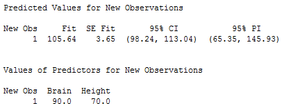
The output reports the 95% prediction interval for an individual college student with brain size = 90 and height = 70. We can be 95% confident that the performance IQ score of an individual college student with brain size = 90 and height = 70 will be between 65.35 and 145.93 counts per 10,000.

When is it okay to use the prediction interval for y_new formula?

The requirements are similar to, but a little more restrictive than, those for the confidence interval. It is okay:

• When \(\textbf{X}_{h}\) is within the "scope of the model." Again, \(\textbf{X}_{h}\) does not have to be an actual observation in the data set.
• When the "LINE" conditions — linearity, independent errors, normal errors, equal error variances — are met. Unlike the case for the formula for the confidence interval, the formula for the prediction interval depends strongly on the condition that the error terms are normally distributed.

Understanding the difference in the two formulas

In our discussion of the confidence interval for µ_Y, we used the formula to investigate what factors affect the width of the confidence interval. There's no need to do it again. Because the formulas are so similar, it turns out that the factors affecting the width of the prediction interval are identical to the factors affecting the width of the confidence interval.

Let's instead investigate the formula for the prediction interval for y_new:

\[\hat{y}_h \pm t_{(\alpha/2, n-(k+1))} \times \sqrt{MSE + [\textrm{se}(\hat{y}_{h})]^2}\]

to see how it compares to the formula for the confidence interval for µ_Y:

\[\hat{y}_h \pm t_{(\alpha/2, n-(k+1))} \times \textrm{se}(\hat{y}_{h})\]

Observe that the only difference in the formulas is that the standard error of the prediction for y_new has an extra MSE term in it that the standard error of the fit for µ_Y does not. If you're not sure why this makes sense, re-read Section 4.11 on "Prediction Interval for a New Response" in the context of simple linear regression.

What's the practical implications of the difference in the two formulas?

• Because the prediction interval has the extra MSE term, a (1-α)100% confidence interval for µ_Y at \(\textbf{X}_{h}\) will always be narrower than the corresponding (1-α)100% prediction interval for y_new at \(\textbf{X}_{h}\).
• By calculating the interval at the sample means of the predictor values and increasing the sample size n, the confidence interval's standard error can approach 0. Because the prediction interval has the extra MSE term, the prediction interval's standard error cannot get close to 0.