8.2 - The Basics of Indicator Variables
A "binary predictor" is a variable that takes on only two possible values. Here are a few common examples of binary predictor variables that you are likely to encounter in your own research:
- Gender (male, female)
- Smoking status (smoker, nonsmoker)
- Treatment (yes, no)
- Health status (diseased, healthy)
- Company status (private, public)
Example: On average, do smoking mothers have babies with lower birth weight?
In the previous section, we briefly investigated data (birthsmokers.txt) on a random sample of n = 32 births that allow researchers (Daniel, 1999) to answer the above research question. The researchers collected the following data:
- Response (y): birth weight (Weight) in grams of baby
- Potential predictor (x1): length of gestation (Gest) in weeks
- Potential predictor (x2): Smoking status of mother (smoker or non-smoker)
In order to include a qualitative variable in a regression model, we have to "code" the variable, that is, assign a unique number to each of the possible categories. A common coding scheme is to use what's called a "zero-one indicator variable." Using such a variable here, we code the binary predictor Smoking as:
- xi2 = 1, if mother i smokes
- xi2 = 0, if mother i does not smoke
In doing so, we use the tradition of assigning the value of 1 to those having the characteristic of interest and 0 to those not having the characteristic. Tradition is less important, though, than making sure you keep track of your coding scheme so that you can properly draw conclusions. Incidentally, other terms sometimes used instead of "zero-one indicator variable" are "dummy variable" or "binary variable".
A scatter plot of the data in which blue circles represent the data on non-smoking mothers (x2=0) and red circles represent the data on smoking mothers (x2=1):
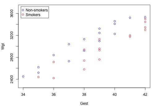
suggests that there might be two distinct linear trends in the data — one for smoking mothers and one for non-smoking mothers. Therefore, a first order model with one binary and one quantitative predictor appears to be a natural model to formulate for these data. That is:
\[y_i=(\beta_0+\beta_1x_{i1}+\beta_2x_{i2})+\epsilon_i\]
where:
- yi is birth weight of baby i in grams
- xi1 is the length of gestation of baby i in weeks
- xi2 = 1, if the mother smoked during pregnancy, and xi2 = 0, if she did not
and the independent error terms εi follow a normal distribution with mean 0 and equal variance σ2.
How does a model containing a (0,1) indicator variable for two groups yield two distinct response functions? In short, this screencast below, illustrates how the mean response function:
\[\mu_Y=\beta_0+\beta_1x_{i1}+\beta_2x_{i2}\]
yields one regression function for non-smoking mothers (xi2 = 0):
\[\mu_Y=\beta_0+\beta_1x_{i1}\]
and one regression function for smoking mothers (xi2 = 1):
\[\mu_Y=(\beta_0+\beta_2)+\beta_1x_{i1}\]
Note that the two formulated regression functions have the same slope (β1) but different intercepts (β0 and β0 + β2) — mathematical characteristics that, based on the above scatter plot, appear to summarize the trend in the data well.
Now, given that we generally use regression models to answer research questions, we need to figure out how each of the parameters in our model enlightens us about our research problem! The fundamental principle is that you can determine the meaning of any regression coefficient by seeing what effect changing the value of the predictor has on the mean response μY. Here's the interpretation of the regression coefficients in a regression model with one (0, 1) binary indicator variable and one quantitative predictor:
- β1 represents the change in the mean response μY for each additional unit increase in the quantitative predictor x1 ... for both groups.
- β2 represents how much higher (or lower) the mean response function of the second group is than that of the first group... for any value of x1.
Upon fitting our formulated regression model to our data, statistical software output tells us:
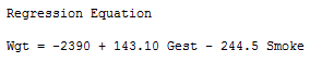
Unfortunately, this output doesn't precede the phrase "regression equation" with the adjective "estimated" in order to emphasize that we've only obtained an estimate of the actual unknown population regression function. But anyway — if we set Smoking once equal to 0 and once equal to 1 — we obtain, as hoped, two distinct estimated lines:
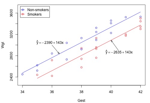
Now, let's use our model and analysis to answer the following research question: Is there a significant difference in mean birth weights for the two groups, after taking into account length of gestation? As is always the case, the first thing we need to do is to "translate" the research question into an appropriate statistical procedure. We can show that if the slope parameter β2 is 0, there is no difference in the means of the two groups — for any length of gestation. That is, we can answer our research question by testing the null hypothesis H0 : β2 = 0 against the alternative HA : β2 ≠ 0.
Well, that's easy enough! The software output:
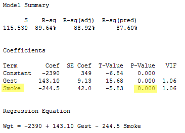
reports that the P-value is < 0.001. At just about any significance level, we can reject the null hypothesis H0 : β2 = 0 in favor of the alternative hypothesis HA : β2 ≠ 0. There is sufficient evidence to conclude that there is a statistically significant difference in the mean birth weight of all babies of smoking mothers and the mean birth weight of babies of all non-smoking mothers, after taking into account length of gestation.
A 95% confidence interval for β2 tells us the magnitude of the difference. A 95% t-multiplier with n-p = 32-3 = 29 degrees of freedom is t(0.025, 29) = 2.0452. Therefore, a 95% confidence interval for β2 is:
-244.54 ± 2.0452(41.98) or (-330.4, -158.7).
We can be 95% confident that the mean birth weight of smoking mothers is between 158.7 and 330.4 grams less than the mean birth weight of non-smoking mothers, for a fixed length of gestation. It is up to the researchers to debate whether or not the difference is a meaningful difference.

