Lesson 11: Introduction to Nonparametric Tests and Bootstrap
Lesson 11: Introduction to Nonparametric Tests and BootstrapOverview
What are Nonparametric Methods?
Nonparametric methods require very few assumptions about the underlying distribution and can be used when the underlying distribution is unspecified.
In the next section, we will focus on inference for one parameter. There are many methods we will not cover for one sample and also many methods for more than one parameter. We present the Sign Test in some detail because it uses many of the concepts we learned in the course. We leave out the details of the other tests.
Objectives
- Determine when to use nonparametric methods.
- Explain how to conduct the Sign test.
- Generate a bootstrap sample.
- Find a confidence interval for any statistic from the bootstrap sample.
11.1 - Inference for the Population Median
11.1 - Inference for the Population MedianIntroduction
So far, the methods we learned were for the population mean. The mean is a good measure of center when the data is bell-shaped, but it is sensitive to outliers and extreme values. When the data is skewed, however, a better measure of center would be the median. The median, you may recall, is a resistant measure. We present an example below that demonstrates why we might consider an alternative method than the one presented so far. In other words, we may want to consider a test for the median and not the mean.
Example 11.1: Tax Forms
The Internal Revenue Service (IRS) claims that it should typically take about 160 minutes to fill out a 1040 tax form. A researcher believes that the IRS's claim is not correct and that it generally takes people longer to complete the form. He recorded the time (in minutes) it took 30 individuals to complete the form. Download the data set: [irs.txt]
How would we approach this using previous methods? We would set the hypotheses as:
\(H_0\colon \mu=160\)
\( H_a\colon \mu>160\)
If we run the analysis in Minitab, we get the following output:
Descriptive Statistics
| N | Mean | StDev | SE Mean | 95% Lower Bound for μ |
|
30 |
209.40 | 159.15 | 29.06 | 160.03 |
μ: mean of time
Test
Alternative hypothesis
H1: μ > 160
| T-Value | P-Value |
|---|---|
| 1.70 | 0.0499 |
The output here gives the \(t\) statistic (1.7001), the degrees of freedom (29) and the p-value (0.04991). In this case, the p-value is less than our significance level, \(\alpha=0.05\). Therefore we reject the null hypothesis and conclude that it takes on average longer than 160 to complete the 1040 form.
We assumed time to fill out the form was Normally distributed (or at least symmetric) BUT time is not Normally distributed (symmetric). It is generally skewed with a long right tail. Let’s take a look at the data. Below is the histogram of the data.
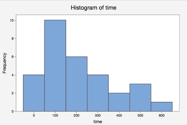
As you can see from the histogram, the shape of the data does not support the assumption that time is Normally distributed. There is a clear right tail here. In a skewed distribution, the population median, typically denoted as \(\eta\), is a better typical value than the population mean, \(\mu\).
11.1.1 - The Sign Test
11.1.1 - The Sign TestSuppose we are interested in testing the population median. The hypotheses are similar to those we have seen before but use the median, \(\eta\), instead of the mean.
If the hypotheses are based on the median, they would look like the following:
Null
- \(H_0\colon\eta=\eta_0\)
Alternative
- \(H_a\colon\eta>\eta_0\)
- \(H_a\colon\eta<\eta_0\)
- \(H_a\colon\eta\ne\eta_0\)
For the IRS example, the null and alternative are:
\(H_0\colon \eta=160\) vs \(H_a\colon \eta >160\)
Consider the test statistic, \(S^+\), where
\(S^+=\text{the number of observations greater than 160}\)
Under the null hypothesis, \(S^+\), should be about 50% of the observations. Therefore, \(S^+\) should have a binomial distribution with parameters \(n\) and \(p=0.5\). Let’s review and verify that it is a Binomial random variable.
- The number of trials, \(n\), is fixed and known. Here the number of trials equals the number of observations. Therefore, in this case, \(n\) is fixed and known.
- The outcomes of each trial can be categorized as either a "success" or a "failure", with the probability of success being \(p\). Observations can either be above the median (a "success") or below the median (a "failure") with the probability of being above the median being \(p=½\).
- The probability of "success" remains constant from trial to trial. The probability of being above the median remains the same for each observation.
- The trials are independent. Each of the observations is independent of the next, so we are okay here.
Now, back to our problem. To make a conclusion, we need to find the p-value. It is the probability of seeing what we see or something more extreme given the null hypothesis is true.
In the IRS example, let’s find \(S^+\), or in other words, let's find the number of observations that fall above 160. We find \(S^+=15\).
Using the Binomial distribution function, we can find the p-value as \(P(S^+\ge 15)\):
\begin{align} P(X\ge15)&=\sum_{i=15}^{30} {30\choose i}(0.5)^{30-i}(0.5)^i\\&=\sum_{i=15}^{30} {30\choose i} (0.5)^{30}\\&\approx 0.5722322 \end{align}
If we assume the significance level is 5%, then the p-value\(>0.05\). We would fail to reject the null hypothesis and conclude that there is no evidence in the data to suggest that the median is above 160 minutes.
This test is called the Sign Test and \(S^+\) is called the sign statistic. The Sign Test is also known as the Binomial Test.
Let's recap what we found. The research question was to see if it took longer than 160 minutes to complete the 1040 form. The measurement was the time in minutes to complete the form. Here is a summary:
|
Assumption |
Test Statistic |
p-value |
Conclusion |
|---|---|---|---|
|
Data are Normally distributed |
t statistic (\(t^*)\) |
0.04991 |
Reject \(H_0\) |
|
Quantitative Data |
Sign statistic \((S^+)\) |
0.572 |
Fail to reject \(H_0\) |
Here, we have two opposite conclusions from each of the tests. Given the shape of the data, which do you think is the valid conclusion?
Minitab®
Minitab Sign Test
We can use Minitab to conduct the Sign test.
- Click Stat > Nonparametrics > 1-Sample sign
- Enter your 'variable', 'significance level', and adjust for the alternative.
- Click OK .
Example 11-2: Tax Forms (Sign Test)
Conduct the test for the median time for filling out the tax forms using the Sign Test in Minitab. Download the dataset: [irs.txt]
Conducting the test in Minitab yields the following output.
1-Sample Sign Test
Method
\(\eta\): median of time
Descriptive Statistics
|
N |
Median |
|
30 |
164 |
95% Lower bound for \(\eta\)
| Lower Bound for \(\eta\) | Achieved Confidence | Position |
| 120.000 | 89.98% |
12 |
| 116.085 | 95.00% | Interpolation |
| 116.000 | 95.06% | 11 |
Test
Alternative hypothesis
H1: \(\eta\) > 160
| Number < 160 | Number = 160 | Number > 160 | P-Value |
|---|---|---|---|
| 15 | 0 | 15 | 0.5722 |
As you can see in the Minitab output, you can also find a confidence interval for the population median based on the sign statistic. As you can imagine, finding the confidence interval by hand is a bit tricky. The interpretation of the confidence interval for the median has the same template interpretation as the confidence interval for the population mean.
We present the details of the Sign Test because it can be found based on the material we covered so far in the course. For the next section, we present another test and how to do it in Minitab but leave out the details.
11.1.2 - One-Sample Wilcoxon
11.1.2 - One-Sample WilcoxonIn this section, we briefly present the one-sample Wilcoxon test. This test was developed by Frank Wilcoxon in 1945. It is considered one of the first “nonparametric” tests developed.
The hypotheses are the similar to the ones presented previously for the Sign Test:
Null
\(H_0\colon \eta=\eta_0\)
Alternative
\(H_a\colon \eta>\eta_0\)
\(H_a\colon \eta<\eta_0\)
\(H_a\colon \eta\ne\eta_0\)
The Wilcoxon test needs additional assumptions, however. They are:
- The random variable of interest is continuous
- The probability distribution of the population is symmetric.
If we compare the assumptions of the Wilcoxon test to the Sign Test, the Wilcoxon test requires the distribution to be symmetric. For example, we should not be making conclusions for the IRS data using the Wilcoxon test because the data is right-skewed.
The test statistic is typically denoted as \(W\). We will not go into details on how this statistic is found as it involves ranks.
Minitab®
One-Sample Wilcoxon Test
Minitab will conduct the one-sample Wilcoxon test.
- Choose Stat > Nonparametrics > 1-sample Wilcoxon
- Enter the 'variable', the 'hypothesized value', and the correct 'alternative'.
- Choose OK .
Example 11-3: Checkout Time (Wilcoxon Test)
Fresh N Friendly food store advertises that their checkout waiting times is four minutes or less. An angry customer wants to dispute this claim. He takes a random sample of shoppers at the peak time and records their checkout times. Can he dispute their claim at significance level 10%?
Checkout times:
3.8, 5.3, 3.5, 4.5, 7.2, 5.1
Use Minitab to conduct the 1-sample Wilcoxon Test. Compare the conclusion to the one found using the one-sample t-test. Lesson 6b.4 More Examples
Wilcoxon Signed Rank Test: time
Method
\(\eta\): median of time
Descriptive Statistics
| Sample |
N |
Median |
|
time |
6 | 4.8 |
Test
Alternative hypothesis
H1: \(\eta\) > 4
N for Wilcoxon
| Sample | N for Test | Wilcoxon Statistic | P-Value |
|---|---|---|---|
| time | 6 | 17.50 | 0.086 |
The p-value for this test is 0.086. The p-value is less than our significance level and therefore we reject the null hypothesis. There is enough evidence in the data to suggest the population median time is greater than 4.
If we assume the data are normal and perform a test for the mean, the p-value was 0.0798.
At the 10% level, the data suggest that both the mean and the median are greater than 4.
11.1.3 - Other Nonparametric Tests
11.1.3 - Other Nonparametric TestsSo far we discussed nonparametric tests for only one parameter. There are many tests for two parameters and for more than two parameters. There are also tests like Fisher’s Exact that will test for the association between two categorical variables.
In the table below, we give some examples of nonparametric tests. If you are interested, explore these tests on your own.
|
Name of Test |
What is used for |
|---|---|
|
Mann-Whitney |
Test for two medians |
|
Wilcoxon Rank-Sum Test |
Test for two paired medians |
|
Kruskal-Wallis |
Test for more than two treatments |
|
Mood’s Median Test |
Test for more than two treatments |
|
Friedman’s Test |
Repeated Measures |
11.2 - Introduction to Bootstrapping
11.2 - Introduction to BootstrappingIn this section, we will start by reviewing the concept of sampling distributions. Recall, we can find the sampling distribution of any summary statistic. Then, the method of bootstrapping samples to find the approximate sampling distribution of a statistic is introduced.
Review of Sampling Distributions
Before looking at the bootstrapping method, we will need to recall the idea of sampling distributions. More specifically, let's look at the sampling distribution of the sample mean, \(\bar{x}\).
Suppose we are interested in estimating the population mean, \(\mu\). To do this, we find a random sample of size \(n\) and calculate the sample mean, \(\bar{x}\). But how do we know how good of an estimate \(\bar{x}\) is? To answer this question, we need to find the standard deviation of the estimate.
Recall that \(\bar{x}\) is calculated from a random sample and is, therefore, a random variable. Let's call the sample mean from above \(\bar{x}_1\). Now suppose we gather another random sample of size \(n\) and calculate \(\bar{x}\) from that sample and denote it \(\bar{x}_2\). Take another sample, and so on and so on. With many of these samples, we can construct a histogram of the sample means.
With theory and the central limit theorem, we have the following summary:
If the sample satisfied at least one of the following:
- The distribution of the random variable, \(X\), is Normal
- The sample size is large; rule of thumb is \(n>30\)
...then the sampling distribution of \(\bar{X}\) is approximately Normal with
- Mean: \(\mu\)
- Standard deviation: \(\frac{\sigma}{\sqrt{n}}\)
- Standard error: \(\frac{s}{\sqrt{n}}\)
Using the above, we can construct confidence intervals, and hypothesis test for the population mean, \(\mu\).
What happens when we do not know the underlying distribution and cannot resample from the distribution? How could we estimate certain sample statistics? This is what we try to answer in the next section.
11.2.1 - Bootstrapping Methods
11.2.1 - Bootstrapping MethodsPoint estimates are helpful to estimate unknown parameters but in order to make inference about an unknown parameter, we need interval estimates. Confidence intervals are based on information from the sampling distribution, including the standard error.
What if the underlying distribution is unknown? What if we are interested in a population parameter that is not the mean, such as the median? How can we construct a confidence interval for the population median?
If we have sample data, then we can use bootstrapping methods to construct a bootstrap sampling distribution to construct a confidence interval.
Bootstrapping is a topic that has been studied extensively for many different population parameters and many different situations. There are parametric bootstrap, nonparametric bootstraps, weighted bootstraps, etc. We merely introduce the very basics of the bootstrap method. To introduce all of the topics would be an entire class in itself.
- Bootstrapping
- Bootstrapping is a resampling procedure that uses data from one sample to generate a sampling distribution by repeatedly taking random samples from the known sample, with replacement.
Let’s show how to create a bootstrap sample for the median. Let the sample median be denoted as \(M\).
- Replace the population with the sample
- Sample with replacement \(B\) times. \(B\) should be large, say 1000.
- Compute sample medians each time, \(M_i\)
- Obtain the approximate distribution of the sample median.
If we have the approximate distribution, we can find an estimate of the standard error of the sample median by finding the standard deviation of \(M_1,...,M_B\).
Sampling with replacement is important. If we did not sample with replacement, we would always get the same sample median as the observed value. The sample we get from sampling from the data with replacement is called the bootstrap sample.
Once we find the bootstrap sample, we can create a confidence interval. For a 90% confidence interval, for example, we would find the 5th percentile and the 95th percentile of the bootstrap sample.
You can create a bootstrap sample to find the approximate sampling distribution of any statistic, not just the median. The steps would be the same except you would calculate the appropriate statistic instead of the median.
Video: Bootstrapping
Sampling R Code from the Bootstrapping Video
sampling.distribution <- function(n = 100, B = 1000, mean = 5, sd = 1, confidence = 0.95) {
  median <- rep(0, B)
  for (i in 1:B) {
    median[i] <- median(rnorm(n, mean = mean, sd = sd))
  }
  med.obs <- median(median)
  c.l <- round((1 - confidence) / 2 * B, 0)
  c.u <- round(B - (1 - confidence) / 2 * B, 0)
  l <- sort(median)[c.l]
  u <- sort(median)[c.u]
  cat(c.l / 1000 * 100, "-percentile:      ", l, "\n")
  cat("Median: ", med.obs, "\n")
  cat(c.u / 1000 * 100, "-percentile:      ", u, "\n")
  return(median)
}

bootstrap.median <- function(data, B = 1000, confidence = 0.95) {
  n <- length(data)
  median <- rep(0, B)
  for (i in 1:B) {
    median[i] <- median(sample(data, size = n, replace = T))
  }
  med.obs <- median(median)
  c.l <- round((1 - confidence) / 2 * B, 0)
  c.u <- round(B - (1 - confidence) / 2 * B, 0)
  l <- sort(median)[c.l]
  u <- sort(median)[c.u]
  cat(c.l / 1000 * 100, "-percentile:      ", l, "\n")
  cat("Median: ", med.obs, "\n")
  cat(c.u / 1000 * 100, "-percentile:      ", u, "\n")
  return(median)
}
11.3 - Summary
11.3 - SummaryIn this Lesson, we introduced the very basic idea behind nonparametric methods. We use nonparametric methods when the assumptions fail for the tests we've learned so far. We also introduced the bootstrap method and how to create a bootstrap sample.