1.5 - Summarizing One Quantitative Variable
1.5 - Summarizing One Quantitative VariableWe will first talk about descriptive measures of quantitative data. The most important characteristic of a data set, central tendency, will be given. After that, a few descriptive measures of the other important characteristic of a data set, the measure of variability, will be discussed. This lesson will be concluded by a discussion of plots, which are simple graphs that show the central location, variability, symmetry, and outliers very clearly.
1.5.1 - Measures of Central Tendency
1.5.1 - Measures of Central TendencyMean, Median, and Mode
A measure of central tendency is an important aspect of quantitative data. It is an estimate of a “typical” value.
Three of the many ways to measure central tendency are the mean, median and mode.
There are other measures, such as a trimmed mean, that we do not discuss here.
- Mean
- The mean is the average of data.
- Sample Mean
- Let $x_1, x_2, \ldots, x_n$ be our sample. The sample mean is usually denoted by $\bar{x}$
- \(\bar{x}=\sum_{i=1}^n \dfrac{x_i}{n}=\dfrac{1}{n}\sum_{i=1}^n x_i\)
- where n is the sample size and \(x_i\) are the measurements. One may need to use the sample mean to estimate the population mean since usually only a random sample is drawn and we don't know the population mean.
The sample mean is a statistic and a population mean is a parameter. Review the definitions of statistic and parameter in Lesson 0.2.
Note on Notation
What if we say we used $y_i$ for our measurements instead of $x_i$? Is this a problem? No. The formula would simply look like this: \(\bar{y}=\sum_{i=1}^n \dfrac{y_i}{n}=\dfrac{1}{n}\sum_{i=1}^n y_i\) The formulas are exactly the same. The letters that you select to denote the measurements are up to you. For instance, many textbooks use $y$ instead of $x$ to denote the measurements. The point is to understand how the calculation that is expressed in the formula works. In this case, the formula is calculating the mean by summing all of the observations and dividing by the number of observations. There is some notation that you will come to see as standards, i.e, n will always equal sample size. We will make a point of letting you know what these are. However, when it comes to the variables, these labels can (and do) vary.
- Median
-
The median is the middle value of the ordered data.
The most important step in finding the median is to first order the data from smallest to largest.
Steps to finding the median for a set of data:
- Arrange the data in increasing order, i.e. smallest to largest.
- Find the location of the median in the ordered data by \(\frac{n+1}{2}\), where n is the sample size.
- The value that represents the location found in Step 2 is the median.
Note on Odd or Even Sample Sizes
If the sample size is an odd number then the location point will produce a median that is an observed value. If the sample size is an even number, then the location will require one to take the mean of two numbers to calculate the median. The result may or may not be an observed value as the example below illustrates.
- Mode
- The mode is the value that occurs most often in the data. It is important to note that there may be more than one mode in the dataset.
Example 1-5: Test Scores
Consider the aptitude test scores of ten children below:
95, 78, 69, 91, 82, 76, 76, 86, 88, 80
Find the mean, median, and mode.
Answer
Mean
\(\bar{x}=\frac{1}{10}(95+78+69+91+82+76+76+86+88+80)=82.1\)
Median
First, order the data.
69, 76, 76, 78, 80, 82, 86, 88, 91, 95
With n = 10, the median position is found by (10 + 1) / 2 = 5.5. Thus, the median is the average of the fifth (80) and sixth (82) ordered value and the median = 81
Mode
The most frequent value in this data set is 76. Therefore the mode is 76.
Effects of Outliers
One shortcoming of the mean is that means are easily affected by extreme values. Measures that are not that affected by extreme values are called resistant. Measures that are affected by extreme values are called sensitive.
Example 1-6: Test Scores Cont'd...
Using the data from Example 1-5, how would the mean and median change, if the entry 91 is mistakenly recorded as 9?
Answer
The data set would be
9, 69, 76, 76, 78, 80, 82, 86, 88, 95
Mean
The mean would be \(\bar{x}=\frac{1}{10}(9+78+69+95+82+76+76+86+88+80)=73.9\)
The mean would be 73.9, which is very different from 82.1.
Median
Let us see the effect of the mistake on the median value.
The data set (with 91 coded as 9) in increasing order is:
9, 69, 76, 76, 78, 80, 82, 86, 88, 95
where the median = 79
The medians of the two sets are not that different. Therefore the median is not that affected by the extreme value 9.
The mean is a sensitive measure (or sensitive statistic) and the median is a resistant measure (or resistant statistic).
After reading this lesson you should know that there are quite a few options when one wants to describe central tendency. In future lessons, we talk about mainly about the mean. However, we need to be aware of one of its shortcomings, which is that it is easily affected by extreme values.
Unless data points are known mistakes, one should not remove them from the data set! One should keep the extreme points and use more resistant measures. For example, use the sample median to estimate the population median. We will discuss methods using the median in Lesson 11.
Adding and Multiplying Constants
What happens to the mean and median if we add or multiply each observation in a data set by a constant?
Consider for example if an instructor curves an exam by adding five points to each student’s score. What effect does this have on the mean and the median? The result of adding a constant to each value has the intended effect of altering the mean and median by the constant.
For example, if in the above example where we have 10 aptitude scores, if 5 was added to each score the mean of this new data set would be 87.1 (the original mean of 82.1 plus 5) and the new median would be 86 (the original median of 81 plus 5).
Similarly, if each observed data value was multiplied by a constant, the new mean and median would change by a factor of this constant. Returning to the 10 aptitude scores, if all of the original scores were doubled, the then the new mean and new median would be double the original mean and median. As we will learn shortly, the effect is not the same on the variance!
Looking Ahead!
Why would you want to know this? One reason, especially for those moving onward to more applied statistics (e.g. Regression, ANOVA), is the transforming data. For many applied statistical methods, a required assumption is that the data is normal, or very near bell-shaped. When the data is not normal, statisticians will transform the data using numerous techniques e.g. logarithmic transformation. We just need to remember the original data was transformed!!
Shape
The shape of the data helps us to determine the most appropriate measure of central tendency. The three most important descriptions of shape are Symmetric, Left-skewed, and Right-skewed. Skewness is a measure of the degree of asymmetry of the distribution.
-
Symmetric
-
- mean, median, and mode are all the same here
- no skewness is apparent
- the distribution is described as symmetric
A symmetrical distribution. -
Left-Skewed or Skewed Left
-
- mean < median
- long tail on the left
A left skewed distribution. -
Right-skewed or Skewed Right
-
- mean > median
- long tail on the right
A right skewed distribution.
Application: The Skewed Nature of Salary Data

Salary distributions are almost always right-skewed, with a few people that make the most money. To illustrate this, consider your favorite sports team or even the company for which you work. There will be one or two players or personnel that earn the “big bucks”, followed by others who earn less. This will produce a shape that is skewed to the right. Knowing this can be a useful aid in negotiating a higher salary.
When one interviews for a position and the discussion gets around to compensation, it is common that the interviewer states an offer that is “typical for someone in your position”. That is, they are offering you the average salary for someone with your particular skill set (e.g. little experience). But is this average the mode, median, or mean? The company – for whom business is business! – will want to pay you the least they can while you prefer to earn the most you can. Since salaries tend to be skewed to the right, the offer will most likely reflect the mode or median. You simply need to ask to which “average” the offer refers and what is the mean of this average since the mean would be the highest of the three values. Once you have these averages, you can begin to negotiate toward the highest number.
1.5.2 - Measures of Position
1.5.2 - Measures of PositionWhile measures of central tendency are important, they do not tell the whole story. For example, suppose the mean score on a statistics exam is 80%. From this information, can we determine a range in which most people scored? The answer is no. There are two other types of measures, measures of position and variability, that help paint a more concise picture of what is going on in the data. In this section, we will consider the measures of position and discuss measures of variability in the next one.
Measures of position give a range where a certain percentage of the data fall. The measures we consider here are percentiles and quartiles.
- Percentiles
- The pth percentile of the data set is a measurement such that after the data are ordered from smallest to largest, at most, p% of the data are at or below this value and at most, (100 - p)% at or above it.
A common application of percentiles is their use in determining passing or failure cutoffs for standardized exams such as the GRE. If you have a 95th percentile score then you are at or above 95% of all test takers.
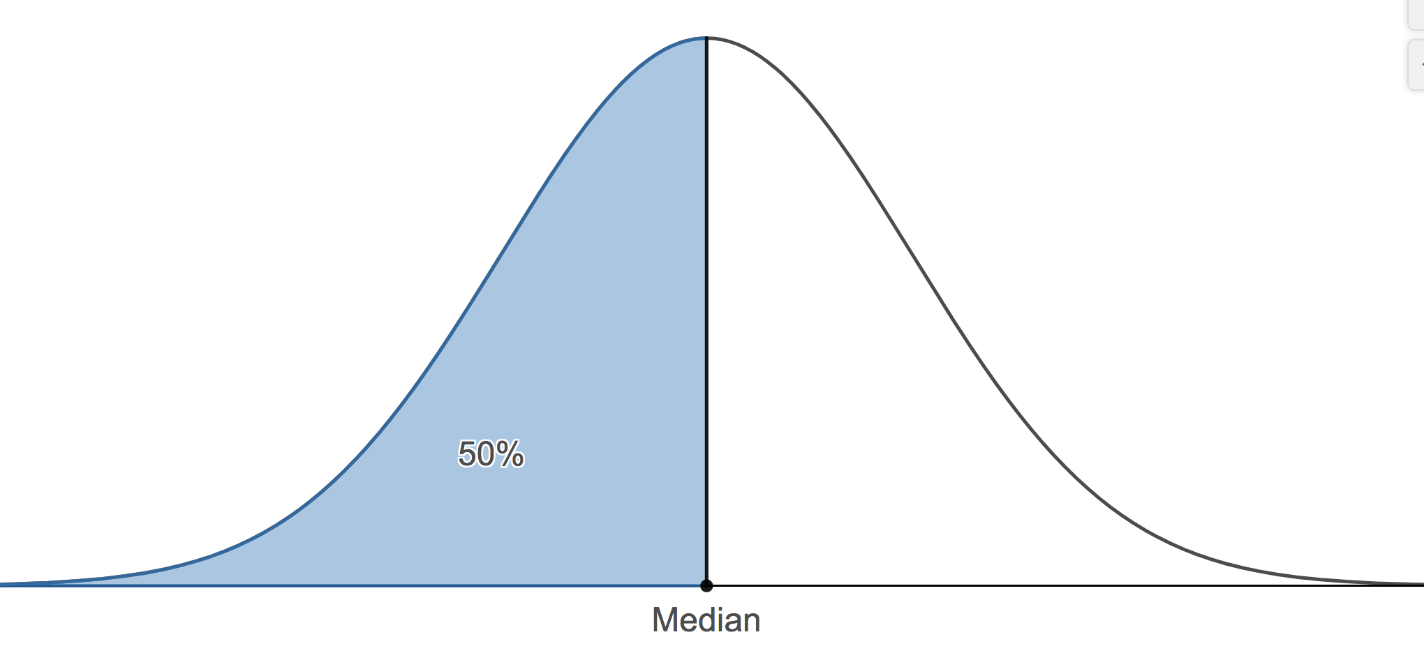
The median is the value where fifty percent or the data values fall at or below it. Therefore, the median is the 50th percentile.
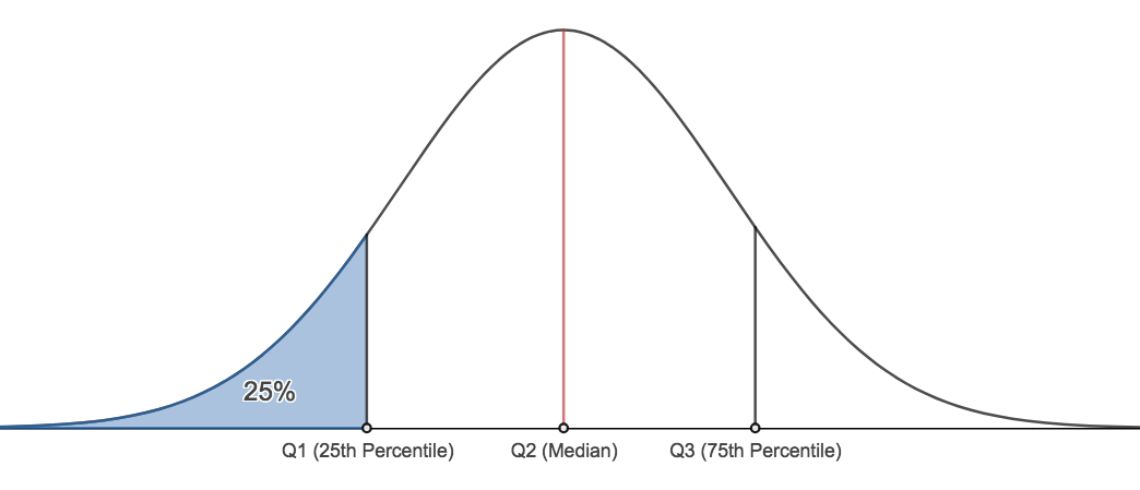
- We can find any percentile we wish. There are two other important percentiles. The 25th percentile, typically denoted, Q1, and the 75th percentile, typically denoted as Q3. Q1 is commonly called the lower quartile and Q3 is commonly called the upper quartile.
Finding Quartiles
The method we will demonstrate for calculating Q1 and Q3 may differ from the method described in our textbook. The results shown here will always be the same as Minitab's results. The method here is also different from the method presented in many undergraduate statistics courses. This method is what we require students to use.
There are two steps to follow:
- Find the location of the desired quartile
If there are n observations, arranged in increasing order, then the first quartile is at position $\dfrac{n+1}{4}$, second quartile (i.e. the median) is at position $\dfrac{2(n+1)}{4}$, and the third quartile is at position $\dfrac{3(n+1)}{4}$.
- Find the value in that position for the ordered data.
Example 1-7: Final Exam Scores
The final exam scores of 18 students are (in increasing order):
24, 58, 61, 67, 71, 73, 76, 79, 82, 83, 85, 87, 88, 88, 92, 93, 94, 97
Find the lower quartile (Q1), the median, and the upper quartile (Q3).
In this example, $n=18$.
For Q1, its position is: $\dfrac{18+1}{4}=4.75$
The actual value of Q1: Q1 = 67 (4th position) + 0.75 · (71 - 67) = 70
For the median, its position is: $\dfrac{18+1}{2}=9.5$
The actual value of the median: Q2 = 82 (9th position) + 0.5 · (83 - 82) = 82.5
For Q3, its position is: \(\dfrac{3(18+1)}{4}=14.25\)
The actual value of Q3: Q3 = 88 + 0.25 · (92 - 88) = 89
The 5 - Number Summary
The Five-Number Summary:
A helpful summary of the data is called the five number summary. The five number summary consists of five values:
- The minimum
- The lower quartile, Q1
- The median (also known as Q2)
- The upper quartile, Q3
- The maximum
Example 1-7
Find the five number summary for the final exam scores. Interpret the values.
\(Min=24, Q1=70, Median=82.5, Q3=89, Max=97\)
The lowest score on the final exam was 24. The highest score on the exam was 97. 25% of the students scored a 70 or below. 50% of the students scored above an 82.5. 75% of the students scored 89 or below. We can also say that 25% of the students scored at least an 89.
1.5.3 - Measures of Variability
1.5.3 - Measures of VariabilityTo introduce the idea of variability, consider this example. Two vending machines A and B drop candies when a quarter is inserted. The number of pieces of candy one gets is random. The following data are recorded for six trials at each vending machine:
Pieces of candy from vending machine A:
1, 2, 3, 3, 5, 4
mean = 3, median = 3, mode = 3
Pieces of candy from vending machine B:
2, 3, 3, 3, 3, 4
mean = 3, median = 3, mode = 3
The dot plot for the pieces of candy from vending machine A and vending machine B is displayed in figure 1.4.
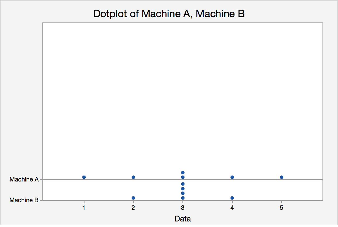
They have the same center, but what about their spreads?
Measures of Variability
There are many ways to describe variability or spread including:
- Range
- Interquartile range (IQR)
- Variance and Standard Deviation
- Range
- The range is the difference in the maximum and minimum values of a data set. The maximum is the largest value in the dataset and the minimum is the smallest value. The range is easy to calculate but it is very much affected by extreme values.
- \(Range = maximum - minimum\)
Like the range, the IQR is a measure of variability, but you must find the quartiles in order to compute its value.
- Interquartile Range (IQR)
- The interquartile range is the difference between upper and lower quartiles and denoted as IQR.
- \begin{align} IQR &=Q3 -Q1\\&=upper\ quartile - lower\ quartile\\&= 75th\ percentile - 25th\ percentile \end{align}
Try it!
Find the IQR for the final exam scores example.
Variance and Standard Deviation
One way to describe spread or variability is to compute the standard deviation. In the following section, we are going to talk about how to compute the sample variance and the sample standard deviation for a data set. The standard deviation is the square root of the variance.
- Variance
- the average squared distance from the mean
- Population variance
- \(\sigma^2=\dfrac{\sum_{i=1}^N (x_i-\mu)^2}{N}\)
- where $\mu$ is the population mean and the summation is over all possible values of the population and \(N\) is the population size.
$\sigma^2$ is often estimated by using the sample variance.
- Sample Variance
- \(s^2=\dfrac{\sum_{i=1}^n (x_i-\bar{x})^2}{n-1}=\dfrac{\sum_{i=1}^n x_i^2-n\bar{x}^2}{n-1}\)
- Where $n$ is the sample size and $\bar{x}$ is the sample mean.
Why do we divide by \(n-1\) instead of by \(n\)?
When we calculate the sample sd we estimate the population mean with the sample mean, and dividing by (n-1) rather than n which gives it a special property that we call an "unbiased estimator". Therefore \(s^2\) is an unbiased estimator for the population variance.
The sample variance (and therefore sample standard deviation) are the common default calculations used by software. When asked to calculate the variance or standard deviation of a set of data, assume - unless otherwise instructed - this is sample data and therefore calculating the sample variance and sample standard deviation.
Example 1-8
Calculate the variance for these final exam scores.
24, 58, 61, 67, 71, 73, 76, 79, 82, 83, 85, 87, 88, 88, 92, 93, 94, 97
First, find the mean:
$\bar{x}=\dfrac{24+58+61+67+71+73+76+79+82+83+85+87+88+88+92+93+94+97}{18}=\dfrac{233}{3}$
|
$x_i$ |
$(x-\bar{x})$ |
$(x-\bar{x})^2$ |
|---|---|---|
|
24 |
-161/3 |
25921/9 |
|
58 |
-59/3 |
3481/9 |
|
61 |
-50/3 |
2500/3 |
|
67 |
-32/3 |
1024/9 |
|
71 |
-20/3 |
400/9 |
|
73 |
-14/3 |
196/9 |
|
76 |
-5/3 |
25/9 |
|
79 |
4/3 |
16/9 |
|
82 |
13/3 |
169/9 |
|
83 |
16/3 |
256/9 |
|
85 |
22/3 |
484/9 |
|
87 |
28/3 |
784/9 |
|
88 |
31/3 |
961/9 |
|
88 |
31/3 |
961/9 |
|
92 |
43/3 |
1849/9 |
|
93 |
46/3 |
2116/9 |
|
94 |
49/3 |
2401/9 |
|
97 |
58/3 |
3364/9 |
|
Sum |
0 |
46908/9 |
Finally,
\(s^2=\dfrac{\sum_{i=1}^n (x_i-\bar{x})^2}{18-1}=\dfrac{46908/9}{17}=\dfrac{5212}{17}\approx 306.588\)
Try it!
Calculate the sample variances for the data set from vending machines A and B yourself and check that it the variance for B is smaller than that for data set A. Work out your answer first, then click the graphic to compare answers.
\(\bar{y}_A=\dfrac{1}{6}(1+2+3+3+5+4)=\dfrac{18}{6}=3\)
\(s^2_A=\dfrac{(1-3)^2+(2-3)^2+(3-3)^2+(3-3)^2+(4-3)^2+(5-3)^2}{6-1}=2\)
\(\bar{y}_B=\dfrac{1}{6}(2+3+3+3+3+4)=\dfrac{18}{6}=3\)
\(s^2_B=\dfrac{(2-3)^2+(3-3)^2+(3-3)^2+(3-3)^2+(3-3)^2+(4-3)^2}{6-1}=0.4\)
Standard Deviation
The standard deviation is a very useful measure. One reason is that it has the same unit of measurement as the data itself (e.g. if a sample of student heights were in inches then so, too, would be the standard deviation. The variance would be in squared units, for example \(inches^2\)). Also, the empirical rule, which will be explained later, makes the standard deviation an important yardstick to find out approximately what percentage of the measurements fall within certain intervals.
- Standard Deviation
- approximately the average distance the values of a data set are from the mean or the square root of the variance
- Population Standard deviation
- \(\sigma=\sqrt{\sigma^2}\)
It has the same unit as the \(x_i\)’s. This is a desirable property since one may think about the spread in terms of the original unit.
\(\sigma\) is estimated by the sample standard deviation \(s\) :
- Sample Standard Deviation
- \(s=\sqrt{s^2}\)
A rough estimate of the standard deviation can be found using \(s\approx \frac{\text{range}}{4}\)
Adding and Multiplying Constants
What happens to measures of variability if we add or multiply each observation in a data set by a constant? We learned previously about the effect such actions have on the mean and the median, but do variation measures behave similarly? Not really.
When we add a constant to all values we are basically shifting the data upward (or downward if we subtract a constant). This has the result of moving the middle but leaving the variability measures (e.g. range, IQR, variance, standard deviation) unchanged.
On the other hand, if one multiplies each value by a constant this does affect measures of variation. The result on the variance is that the new variance is multiplied by the square of the constant, while the standard deviation, range, and IQR are multiplied by the constant. For example, if the observed values of Machine A in the example above were multiplied by three, the new variance would be 18 (the original variance of 2 multiplied by 9). The new standard deviation would be 4.242 (the original standard 1.414 multiplied by 3). The range and IQR would also change by a factor of 3.
Coefficient of Variation
Above we considered three measures of variation: Range, IQR, and Variance (and its square root counterpart - Standard Deviation). These are all measures we can calculate from one quantitative variable e.g. height, weight. But how can we compare dispersion (i.e. variability) of data from two or more distinct populations that have vastly different means?
A popular statistic to use in such situations is the Coefficient of Variation or CV. This is a unit-free statistic and one where the higher the value the greater the dispersion. The calculation of CV is:
- Coefficient of Variation (CV)
- \(CV = \dfrac{\text{Standard Deviation}}{\text{Mean}}\)
To demonstrate, think of prices for luxury and budget hotels. Which do you think would have the higher average cost per night? Which would have the greater standard deviation? The CV would allow you to compare this dispersion in costs in relative terms by accounting for the fact that the luxury hotels would have a greater mean and standard deviation.
Example 1-9: Comparing Prices
You are shopping for toilet tissue. As you compare prices of various brands, some offer price per roll while others offer price per sheet. You are interested in determining which pricing method has less variability so you sample several of each and calculate the mean and standard deviation for the sampled items that are priced per roll, and the mean and standard deviation for the sampled items that are priced per sheet. The table below summarizes your results.
|
Item |
Mean |
Standard Deviation |
|---|---|---|
|
Price per Roll |
0.9196 |
0.4233 |
|
Price Per Sheet |
0.01134 |
0.00553 |
Comparing the standard deviations the Per Sheet appears to have much less variability in pricing. However, the mean is also much smaller. The coefficient of variation allows us to make a relative comparison of the variability of these two pricing schemes:
\(CV_{roll}=\dfrac{0.4233}{0.9196}=0.46\)
\(CV_{sheet}=\dfrac{0.00553}{0.01134}=0.49\)
Relatively speaking, the variation for Price per Sheet is greater than the variability for Price per Roll.
1.5.4 - Minitab: Descriptive Statistics
1.5.4 - Minitab: Descriptive StatisticsMinitab®
Descriptive Statistics
Let's perform some basic operations in Minitab. Some of the examples below are repeats of what we did by hand in earlier lessons while others are new. First, we saw previously how you can enter data into the Minitab worksheet by hand, we will now walk through how to load a dataset into Minitab from an Excel file.
Loading Data into Minitab from an Excel File
For the examples in this section, download the minitabintrodata.xlsx spreadsheet file. Save the file locally (if using Minitab installed on the computer you are using).
Open Minitab web and choose 'Open Local File' to find the spreadsheet file.
With the data in the Minitab worksheet, you can then perform any number of procedures. First, we obtain some basic descriptive statistics.
Descriptive Statistics
With the data from the Excel spreadsheet file into your Minitab worksheet window, you should notice that all columns are labeled ‘Cx’ where the ‘x’ is a number. Some of these are followed by a ‘-T’. Those columns with the ‘-T’ indicate that the data in this column are considered text or categorical data. Otherwise, Minitab recognizes the data as quantitative. If the operation you conduct in Minitab only functions on a certain variable type (e.g. calculating the mean can only be done on quantitative data) then only columns of that data type will be available to use for those operations.
Minitab®
Example 1-10 Hours Data
Let's use Minitab to calculate the five number summary, mean and standard deviation for the Hours data, (contained in minitabintrodata.xlsx). And, as you will see, Minitab by default will provide some added information.
1. At top of the Minitab window select the menu option Stat > Basic Statistics > Display Descriptive Statistics
2. Once this dialog box opens your cursor should be blinking in the 'Variables' window. If not, simply click inside this part of the dialog box. The only variables you should see in the left side window are columns of quantitative data (the two price columns, age, and hours). To enter a variable from the left hand window into the Variables window you can either double-click that variable or click the variable to highlight it and then click the 'Select' button. Do so with the variable 'Hours'.
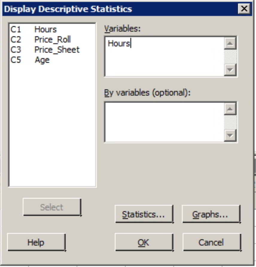
3. With the variable 'Hours' in the 'Variable' window click the 'OK' button.
The following output should appear in the Session window above the worksheet.
Statistics
Variable | N | N* | Mean | SE Mean | StDev | Minimum | Q1 | Median | Q3 | Maximum |
|---|---|---|---|---|---|---|---|---|---|---|
Hours | 50 | 835 | 16.00 | 1.19 | 8.45 | 4.00 | 9.00 | 15.00 | 22.25 | 34.00 |
The mean, standard deviation (StDev), etc. should be the same values as those calculated in the practice problems. Minitab also gives the size of the sample used to create these statistics (N), and the number of observations from this data that were missing (N*).
These statistics are the default statistics. Additional basic descriptive statistics are also available such as trim mean and coefficient of variation (CV).
Minitab®
Example 1-11: The Coefficient of Variation (CV)
To get the CV values for the Price per Sheet and Price per Roll an example found in an earlier lesson, (data contained in minitabintrodata.xlsx).
- Open Minitab and return to Stat > Basic Statistics > Display Descriptive Statistics.
- Enter both variables into the Variables window. That is, both 'Price_Roll' and 'Price_Sheet' should be in the Variables window.
- Click the Statistics tab and then check the box for 'Coefficient of Variation' (notice the other statistics available!) and click OK.
- Click OK again.
The output will include the same statistics as the example above plus the CV values, (it will be titled 'CoefVar').
Descriptive Statistics: Price_Roll, Price_Sheet
Statistics
Variable | N | N* | Mean | SE Mean | StDev | CoefVar | Minimum | Q1 | Median | Q3 | Maximum |
|---|---|---|---|---|---|---|---|---|---|---|---|
Price_Roll | 24 | 861 | 0.9196 | 0.0864 | 0.4233 | 46.03 | 0.5300 | 0.6075 | 0.7750 | 0.9500 | 1.9800 |
Price_Sheet | 24 | 861 | 0.01134 | 0.00113 | 0.00553 | 48.78 | 0.00610 | 0.00753 | 0.00995 | 0.01490 | 0.03180 |