Lesson 6: MLR Model Evaluation
Lesson 6: MLR Model EvaluationOverview
For the simple linear regression model, there is only one slope parameter about which one can perform hypothesis tests. For the multiple linear regression model, there are three different hypothesis tests for slopes that one could conduct. They are:
- a hypothesis test for testing that one slope parameter is 0
- a hypothesis test for testing that all of the slope parameters are 0
- a hypothesis test for testing that a subset — more than one, but not all — of the slope parameters are 0
In this lesson, we learn how to perform each of the above three hypothesis tests. Along the way, however, we have to take two asides — one to learn about the "general linear F-test" and one to learn about "sequential sums of squares." Knowledge about both is necessary for performing the three hypothesis tests.
Objectives
- Translate research questions involving slope parameters into the appropriate hypotheses for testing.
- Understand the general idea behind the general linear test.
- Calculate a sequential sum of squares using either of the two definitions.
- Know how to obtain a two (or more)-degree-of-freedom sequential sum of squares.
- Know how to calculate a partial F-statistic from sequential sums of squares.
- Understand the decomposition of a regression sum of squares into a sum of sequential sums of squares.
- Understand that the t-test for a slope parameter tests the marginal significance of the predictor after adjusting for the other predictors in the model (as can be justified by the equivalence of the t-test and the corresponding partial F-test for one slope).
- Perform a general hypothesis test using the general linear test and relevant Minitab output.
- Know how to specify the null and alternative hypotheses and be able to draw a conclusion given appropriate Minitab output for the t-test or partial F-test for \(H_{0} \colon \beta_k = 0\).
- Know how to specify the null and alternative hypotheses and be able to draw a conclusion given appropriate Minitab output for the overall F-test for \(H_{0 } \colon \beta_1 \dots \beta_{p-1} = 0\)
- Know how to specify the null and alternative hypotheses and be able to draw a conclusion given appropriate Minitab output for the partial F-test for any subset of the slope parameters.
- Calculate and understand partial \(R^{2}\).
Lesson 6 Code Files
Below is a zip file that contains all the data sets used in this lesson:
- alcoholarm.txt
- allentest.txt
- coolhearts.txt
- iqsize.txt
- peru.txt
- Physical.txt
- sugarbeets.txt
6.1 - Three Types of Hypotheses
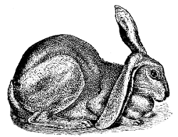
6.1 - Three Types of HypothesesExample 6-1: Heart attacks in Rabbits
Let's investigate an example that highlights the differences between the three hypotheses that we will learn how to test in this lesson.
When the heart muscle is deprived of oxygen, the tissue dies and leads to a heart attack ("myocardial infarction"). Apparently, cooling the heart reduces the size of the heart attack. It is not known, however, whether cooling is only effective if it takes place before the blood flow to the heart becomes restricted. Some researchers (Hale, et al, 1997) hypothesized that cooling the heart would be effective in reducing the size of the heart attack even if it takes place after the blood flow becomes restricted.
To investigate their hypothesis, the researchers conducted an experiment on 32 anesthetized rabbits that were subjected to a heart attack. The researchers established three experimental groups:
- Rabbits whose hearts were cooled to 6º C within 5 minutes of the blocked artery ("early cooling")
- Rabbits whose hearts were cooled to 6º C within 25 minutes of the blocked artery ("late cooling")
- Rabbits whose hearts were not cooled at all ("no cooling")
At the end of the experiment, the researchers measured the size of the infarcted (i.e., damaged) area (in grams) in each of the 32 rabbits. But, as you can imagine, there is great variability in the size of hearts. The size of a rabbit's infarcted area may be large only because it has a larger heart. Therefore, in order to adjust for differences in heart sizes, the researchers also measured the size of the region at risk for infarction (in grams) in each of the 32 rabbits.
With their measurements in hand (Cool Hearts data), the researchers' primary research question was:
Does the mean size of the infarcted area differ among the three treatment groups — no cooling, early cooling, and late cooling — when controlling for the size of the region at risk for infarction?
A regression model that the researchers might use in answering their research question is:
\(y_i=(\beta_0+\beta_1x_{i1}+\beta_2x_{i2}+\beta_3x_{i3})+\epsilon_i\)
where:
- \(y_{i}\) is the size of the infarcted area (in grams) of rabbit i
- \(x_{i1}\) is the size of the region at risk (in grams) of rabbit i
- \(x_{i2}\) = 1 if early cooling of rabbit i, 0 if not
- \(x_{i3}\) = 1 if late cooling of rabbit i, 0 if not
and the independent error terms \(\epsilon_{i}\) follow a normal distribution with mean 0 and equal variance \(σ^{2}\).
The predictors \(x_{2}\) and \(x_{3}\) are "indicator variables" that translate the categorical information on the experimental group to which a rabbit belongs into a usable form. We'll learn more about such variables in Lesson 8, but for now observe that for "early cooling" rabbits \(x_{2}\) = 1 and \(x_{3}\) = 0, for "late cooling" rabbits \(x_{2}\) = 0 and \(x_{3}\) = 1, and for "no cooling" rabbits \(x_{2}\) = 0 and \(x_{3}\) = 0. The model can therefore be simplified for each of the three experimental groups:
| Early Cooling | \(y_i=(\beta_0+\beta_1x_{i1}+\beta_2)+\epsilon_i\) |
|---|---|
| Late Cooling | \(y_i=(\beta_0+\beta_1x_{i1}+\beta_3)+\epsilon_i\) |
| No Cooling | \(y_i=(\beta_0+\beta_1x_{i1})+\epsilon_i\) |
Thus, \(\beta_2\) represents the difference in the mean size of the infarcted area — controlling for the size of the region at risk —between "early cooling" and "no cooling" rabbits. Similarly, \(\beta_3\) represents the difference in the mean size of the infarcted area — controlling for the size of the region at risk —between "late cooling" and "no cooling" rabbits.
Fitting the above model to the researchers' data, Minitab reports:
Regression Equation
Inf = -0.135 + 0.613 Area - 0.2435 X2 - 0.0657 X3
A plot of the data adorned with the estimated regression equation looks like this:
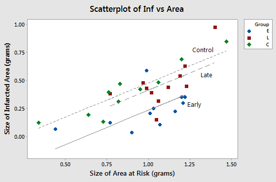
The plot suggests that, as we'd expect, as the size of the area at risk increases, the size of the infarcted area also tends to increase. The plot also suggests that for this sample of 32 rabbits with a given size of area at risk, 1.0 grams for example, the average size of the infarcted area differs for the three experimental groups. But, the researchers aren't just interested in this sample. They want to be able to answer their research question for the whole population of rabbits.
How could the researchers use the above regression model to answer their research question? Note that the estimated slope coefficients \(b_{2}\) and \(b_{3}\) are -0.2435 and -0.0657, respectively. If the estimated coefficients \(b_{2}\) and \(b_{3}\) were instead both 0, then the average size of the infarcted area would be the same for the three groups of rabbits in this sample. It can be shown that the mean size of the infarcted area would be the same for the whole population of rabbits — controlling for the size of the region at risk — if the two slopes \(\beta_{2}\) and \(\beta_{3}\) simultaneously equal 0. That is, the researchers's question reduces to testing the hypothesis \(H_{0}\colon \beta_{2} = \beta_{3} = 0\).
I'm hoping this example clearly illustrates the need for being able to "translate" a research question into a statistical procedure. Often, the procedure involves four steps, namely:
- formulating a multiple regression model
- determining how the model helps answer the research question
- checking the model
- and performing a hypothesis test (or calculating a confidence interval)
In this lesson, we learn how to perform three different hypothesis tests for slope parameters in order to answer various research questions. Let's take a look at the different research questions — and the hypotheses we need to test in order to answer the questions — for our heart attacks in rabbits example.
A research question
Consider the research question: "Is a regression model containing at least one predictor useful in predicting the size of the infarct?" Are you convinced that testing the following hypotheses helps answer the research question?
- \(H_{0}\colon \beta_{1} = \beta_{2} = \beta_{3} = 0\)
- \(H_{A}\colon\) At least one \(\beta_{i} \ne 0\) (for i = 1, 2, 3)
In this case, the researchers are interested in testing that all three slope parameters are zero. We'll soon see that the null hypothesis is tested using the analysis of variance F-test.
Another research question
Consider the research question: "Is the size of the infarct significantly (linearly) related to the area of the region at risk?" Are you convinced that testing the following hypotheses helps answer the research question?
- \(H_{0} \colon \beta_{1} = 0\)
- \(H_{A} \colon \beta_{1} ≠ 0\)
In this case, the researchers are interested in testing that just one of the three slope parameters is zero. You already know how to do this, don't you? Wouldn't this just involve performing a t-test for \(\beta_{1}\)? We'll soon learn how to think about the t-test for a single slope parameter in the multiple regression framework.
A final research question
Consider the researcher's primary research question: "Is the size of the infarct area significantly (linearly) related to the type of treatment after controlling for the size of the region at risk for infarction?" Are you convinced that testing the following hypotheses helps answer the research question?
- \(H_{0} \colon \beta_{2} = \beta_{3} = 0\)
- \(H_{A} \colon\) At least one \(\beta_{i} ≠ 0\) (for i = 2, 3)
In this case, the researchers are interested in testing whether a subset (more than one, but not all) of the slope parameters are simultaneously zero. We will learn a general linear F-test for testing such a hypothesis.
Unfortunately, we can't just jump right into the hypothesis tests. We first have to take two side trips — the first one to learn what is called "the general linear F-test."
6.2 - The General Linear F-Test
6.2 - The General Linear F-TestThe General Linear F-Test
The "general linear F-test" involves three basic steps, namely:
- Define a larger full model. (By "larger," we mean one with more parameters.)
- Define a smaller reduced model. (By "smaller," we mean one with fewer parameters.)
- Use an F-statistic to decide whether or not to reject the smaller reduced model in favor of the larger full model.
As you can see by the wording of the third step, the null hypothesis always pertains to the reduced model, while the alternative hypothesis always pertains to the full model.
The easiest way to learn about the general linear test is to first go back to what we know, namely the simple linear regression model. Once we understand the general linear test for the simple case, we then see that it can be easily extended to the multiple-case model. We take that approach here.
The Full Model
The "full model", which is also sometimes referred to as the "unrestricted model," is the model thought to be most appropriate for the data. For simple linear regression, the full model is:
\(y_i=(\beta_0+\beta_1x_{i1})+\epsilon_i\)
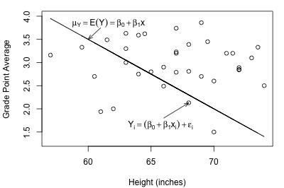
Here's a plot of a hypothesized full model for a set of data that we worked with previously in this course (student heights and grade point averages):
And, here's another plot of a hypothesized full model that we previously encountered (state latitudes and skin cancer mortalities):
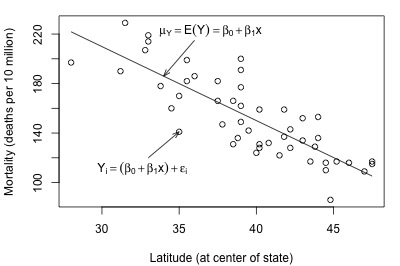
In each plot, the solid line represents what the hypothesized population regression line might look like for the full model. The question we have to answer in each case is "does the full model describe the data well?" Here, we might think that the full model does well in summarizing the trend in the second plot but not the first.
The Reduced Model
The "reduced model," which is sometimes also referred to as the "restricted model," is the model described by the null hypothesis \(H_{0}\). For simple linear regression, a common null hypothesis is \(H_{0} : \beta_{1} = 0\). In this case, the reduced model is obtained by "zeroing out" the slope \(\beta_{1}\) that appears in the full model. That is, the reduced model is:
\(y_i=\beta_0+\epsilon_i\)
This reduced model suggests that each response \(y_{i}\) is a function only of some overall mean, \(\beta_{0}\), and some error \(\epsilon_{i}\).
Let's take another look at the plot of student grade point average against height, but this time with a line representing what the hypothesized population regression line might look like for the reduced model:
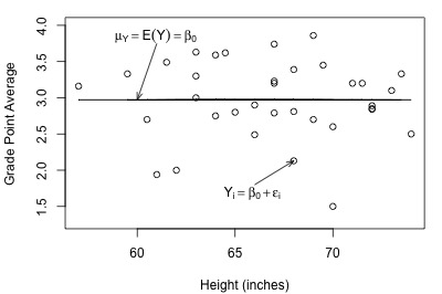
Not bad — there (fortunately?!) doesn't appear to be a relationship between height and grade point average. And, it appears as if the reduced model might be appropriate in describing the lack of a relationship between heights and grade point averages. What does the reduced model do for the skin cancer mortality example?
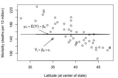
It doesn't appear as if the reduced model would do a very good job of summarizing the trend in the population.
F-Statistic Test
How do we decide if the reduced model or the full model does a better job of describing the trend in the data when it can't be determined by simply looking at a plot? What we need to do is to quantify how much error remains after fitting each of the two models to our data. That is, we take the general linear test approach:
- "Fit the full model" to the data.
- Obtain the least squares estimates of \(\beta_{0}\) and \(\beta_{1}\).
- Determine the error sum of squares, which we denote as "SSE(F)."
- "Fit the reduced model" to the data.
- Obtain the least squares estimate of \(\beta_{0}\).
- Determine the error sum of squares, which we denote as "SSE(R)."
Recall that, in general, the error sum of squares is obtained by summing the squared distances between the observed and fitted (estimated) responses:
\(\sum(\text{observed } - \text{ fitted})^2\)
Therefore, since \(y_i\) is the observed response and \(\hat{y}_i\) is the fitted response for the full model:
\(SSE(F)=\sum(y_i-\hat{y}_i)^2\)
And, since \(y_i\) is the observed response and \(\bar{y}\) is the fitted response for the reduced model:
\(SSE(R)=\sum(y_i-\bar{y})^2\)
Let's get a better feel for the general linear F-test approach by applying it to two different datasets. First, let's look at the Height and GPA data. The following plot of grade point averages against heights contains two estimated regression lines — the solid line is the estimated line for the full model, and the dashed line is the estimated line for the reduced model:
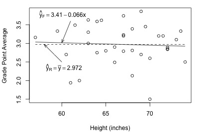
As you can see, the estimated lines are almost identical. Calculating the error sum of squares for each model, we obtain:
\(SSE(F)=\sum(y_i-\hat{y}_i)^2=9.7055\)
\(SSE(R)=\sum(y_i-\bar{y})^2=9.7331\)
The two quantities are almost identical. Adding height to the reduced model to obtain the full model reduces the amount of error by only 0.0276 (from 9.7331 to 9.7055). That is, adding height to the model does very little in reducing the variability in grade point averages. In this case, there appears to be no advantage in using the larger full model over the simpler reduced model.
Look what happens when we fit the full and reduced models to the skin cancer mortality and latitude dataset:
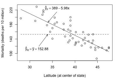
Here, there is quite a big difference between the estimated equation for the full model (solid line) and the estimated equation for the reduced model (dashed line). The error sums of squares quantify the substantial difference in the two estimated equations:
\(SSE(F)=\sum(y_i-\hat{y}_i)^2=17173\)
\(SSE(R)=\sum(y_i-\bar{y})^2=53637\)
Adding latitude to the reduced model to obtain the full model reduces the amount of error by 36464 (from 53637 to 17173). That is, adding latitude to the model substantially reduces the variability in skin cancer mortality. In this case, there appears to be a big advantage in using the larger full model over the simpler reduced model.
Where are we going with this general linear test approach? In short:
- The general linear test involves a comparison between SSE(R) and SSE(F).
- SSE(R) can never be smaller than SSE(F). It is always larger than (or possibly the same as) SSE(F).
- If SSE(F) is close to SSE(R), then the variation around the estimated full model regression function is almost as large as the variation around the estimated reduced model regression function. If that's the case, it makes sense to use the simpler reduced model.
- On the other hand, if SSE(F) and SSE(R) differ greatly, then the additional parameter(s) in the full model substantially reduce the variation around the estimated regression function. In this case, it makes sense to go with the larger full model.
How different does SSE(R) have to be from SSE(F) in order to justify using the larger full model? The general linear F-statistic:
\(F^*=\left( \dfrac{SSE(R)-SSE(F)}{df_R-df_F}\right)\div\left( \dfrac{SSE(F)}{df_F}\right)\)
helps answer this question. The F-statistic intuitively makes sense — it is a function of SSE(R)-SSE(F), the difference in the error between the two models. The degrees of freedom — denoted \(df_{R}\) and \(df_{F}\) — are those associated with the reduced and full model error sum of squares, respectively.
We use the general linear F-statistic to decide whether or not:
- to reject the null hypothesis \(H_{0}\colon\) The reduced model
- in favor of the alternative hypothesis \(H_{A}\colon\) The full model
In general, we reject \(H_{0}\) if F* is large — or equivalently if its associated P-value is small.
The test applied to the simple linear regression model
For simple linear regression, it turns out that the general linear F-test is just the same ANOVA F-test that we learned before. As noted earlier for the simple linear regression case, the full model is:
\(y_i=(\beta_0+\beta_1x_{i1})+\epsilon_i\)
and the reduced model is:
\(y_i=\beta_0+\epsilon_i\)
Therefore, the appropriate null and alternative hypotheses are specified either as:
- \(H_{0} \colon y_i = \beta_{0} + \epsilon_{i}\)
- \(H_{A} \colon y_i = \beta_{0} + \beta_{1} x_{i} + \epsilon_{i}\)
or as:
- \(H_{0} \colon \beta_{1} = 0 \)
- \(H_{A} \colon \beta_{1} ≠ 0 \)
The degrees of freedom associated with the error sum of squares for the reduced model is n-1, and:
\(SSE(R)=\sum(y_i-\bar{y})^2=SSTO\)
The degrees of freedom associated with the error sum of squares for the full model is n-2, and:
\(SSE(F)=\sum(y_i-\hat{y}_i)^2=SSE\)
Now, we can see how the general linear F-statistic just reduces algebraically to the ANOVA F-test that we know:
\(F^*=\left( \dfrac{SSE(R)-SSE(F)}{df_R-df_F}\right)\div\left( \dfrac{SSE(F)}{df_F}\right)\)
Can be rewritten by substituting...
\(\begin{aligned} &&df_{R} = n - 1\\ &&df_{F} = n - 2\\ &&SSE(R)=SSTO\\&&SSE(F)=SSE\end{aligned}\)
\(F^*=\left( \dfrac{SSTO-SSE}{(n-1)-(n-2)}\right)\div\left( \dfrac{SSE}{(n-2)}\right)=\frac{MSR}{MSE}\)
That is, the general linear F-statistic reduces to the ANOVA F-statistic:
\(F^*=\dfrac{MSR}{MSE}\)
For the student height and grade point average example:
\( F^*=\dfrac{MSR}{MSE}=\dfrac{0.0276/1}{9.7055/33}=\dfrac{0.0276}{0.2941}=0.094\)
For the skin cancer mortality example:
\( F^*=\dfrac{MSR}{MSE}=\dfrac{36464/1}{17173/47}=\dfrac{36464}{365.4}=99.8\)
The P-value is calculated as usual. The P-value answers the question: "what is the probability that we’d get an F* statistic as large as we did if the null hypothesis were true?" The P-value is determined by comparing F* to an F distribution with 1 numerator degree of freedom and n-2 denominator degrees of freedom. For the student height and grade point average example, the P-value is 0.761 (so we fail to reject \(H_{0}\) and we favor the reduced model), while for the skin cancer mortality example, the P-value is 0.000 (so we reject \(H_{0}\) and we favor the full model).
Example 6-2: Alcohol and muscle Strength
Does alcoholism have an effect on muscle strength? Some researchers (Urbano-Marquez, et al, 1989) who were interested in answering this question collected the following data (Alcohol Arm data) on a sample of 50 alcoholic men:
- x = the total lifetime dose of alcohol (kg per kg of body weight) consumed
- y = the strength of the deltoid muscle in the man's non-dominant arm
The full model is the model that would summarize a linear relationship between alcohol consumption and arm strength. The reduced model, on the other hand, is the model that claims there is no relationship between alcohol consumption and arm strength.
Therefore, the appropriate null and alternative hypotheses are specified either as:
- \(H_0 \colon y_i = \beta_0 + \epsilon_i \)
- \(H_A \colon y_i = \beta_0 + \beta_{1}x_i + \epsilon_i\)
or as:
- \(H_0 \colon \beta_1 = 0\)
- \(H_A \colon \beta_1 ≠ 0\)
Upon fitting the reduced model to the data, we obtain:
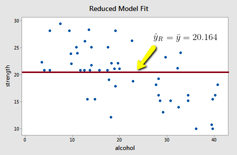
and:
\(SSE(R)=\sum(y_i-\bar{y})^2=1224.32\)
Note that the reduced model does not appear to summarize the trend in the data very well.
Upon fitting the full model to the data, we obtain:
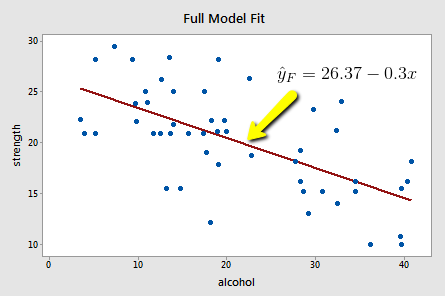
and:
\(SSE(F)=\sum(y_i-\hat{y}_i)^2=720.27\)
The full model appears to describe the trend in the data better than the reduced model.
The good news is that in the simple linear regression case, we don't have to bother with calculating the general linear F-statistic. Minitab does it for us in the ANOVA table.
Click on the light bulb
Analysis of Variance
| Source | DF | Adj SS | Adj MS | F-Value | P-Value |
|---|---|---|---|---|---|
| Regression | 1 | 504.04 | 504.040 | 33.5899 | 0.000 |
| Error | 48 | 720.27 | 15.006 | ||
| Total | 49 | 1224.32 |
As you can see, Minitab calculates and reports both SSE(F) — the amount of error associated with the full model — and SSE(R) — the amount of error associated with the reduced model. The F-statistic is:
\( F^*=\dfrac{MSR}{MSE}=\dfrac{504.04/1}{720.27/48}=\dfrac{504.04}{15.006}=33.59\)
and its associated P-value is < 0.001 (so we reject \(H_{0}\) and favor the full model). We can conclude that there is a statistically significant linear association between lifetime alcohol consumption and arm strength.
This concludes our discussion of our first aside from the general linear F-test. Now, we move on to our second aside from sequential sums of squares.
6.3 - Sequential (or Extra) Sums of Squares
6.3 - Sequential (or Extra) Sums of SquaresThe numerator of the general linear F-statistic — that is, \(SSE(R)-SSE(F)\) is what is referred to as a "sequential sum of squares" or "extra sum of squares."
Definition
- What is a "sequential sum of squares?"
- It can be viewed in either of two ways:
- It is the reduction in the error sum of squares (SSE) when one or more predictor variables are added to the model.
- Or, it is the increase in the regression sum of squares (SSR) when one or more predictor variables are added to the model.
In essence, when we add a predictor to a model, we hope to explain some of the variability in the response, and thereby reduce some of the error. A sequential sum of squares quantifies how much variability we explain (increase in regression sum of squares) or alternatively how much error we reduce (reduction in the error sum of squares).
Notation
The amount of error that remains upon fitting a multiple regression model naturally depends on which predictors are in the model. That is, the error sum of squares (SSE) and, hence, the regression sum of squares (SSR) depend on what predictors are in the model. Therefore, we need a way of keeping track of the predictors in the model for each calculated SSE and SSR value.
We'll just note what predictors are in the model by listing them in parentheses after any SSE or SSR. For example:
- \(SSE({x}_{1})\) denotes the error sum of squares when \(x_{1}\) is the only predictor in the model.
- \(SSR({x}_{1}, {x}_{2})\) denotes the regression sum of squares when \(x_{1}\) and \(x_{2}\) are both in the model.
And, we'll use notation like \(SSR(x_{2} | x_{1})\) to denote a sequential sum of squares. \(SSR(x_{2} | x_{1})\) denotes the sequential sum of squares obtained by adding \(x_{2}\) to a model already containing only the predictor \(x_{1}\). The vertical bar "|" is read as "given" — that is, "\(x_{2}\) | \(x_{1}\)" is read as "\(x_{2}\) given \(x_{1}\)." In general, the variables appearing to the right of the bar "|" are the predictors in the original model, and the variables appearing to the left of the bar "|" are the predictors newly added to the model.
Here are a few more examples of the notation:
- The sequential sum of squares obtained by adding \(x_{1}\) to the model already containing only the predictor \(x_{2}\) is denoted as \(SSR({x}_{1}| {x}_{2})\).
- The sequential sum of squares obtained by adding \(x_{1}\) to the model in which \(x_{2}\) and \(x_{3}\) are predictors is denoted as \(SSR({x}_{1}| {x}_{2},{x}_{3}) \).
- The sequential sum of squares obtained by adding \(x_{1}\) and \(x_{2}\) to the model in which \(x_{3}\) is the only predictor is denoted as \(SSR({x}_{1}, {x}_{2}|{x}_{3}) \).
Let's try out the notation and the two alternative definitions of a sequential sum of squares on an example.
Example 6-3: ACL Test Scores
In the Allen Cognitive Level (ACL) Study, David and Riley (1990) investigated the relationship between ACL test scores and level of psychopathology. They collected the following data (Allen Test dataset) on each of the 69 patients in a hospital psychiatry unit:
- Response y = ACL score
- Potential predictor \(x_{1}\) = vocabulary ("Vocab") score on Shipley Institute of Living Scale
- Potential predictor \(x_{2}\) = abstraction ("Abstract") score on Shipley Institute of Living Scale
- Potential predictor \(x_{3}\) = score on Symbol-Digit Modalities Test ("SDMT")
If we estimate the regression function with y = ACL as the response and \(x_{1}\) = Vocab as the predictor, that is, if we "regress y = ACL on \(\boldsymbol{x_{1}}\) = Vocab," we obtain:
Analysis of Variance
| Source | DF | Adj SS | Adj MS | F-Value | P-Value |
|---|---|---|---|---|---|
| Regression | 1 | 2.691 | 2.6906 | 4.47 | 0.038 |
| Vocab | 1 | 2.691 | 2.6909 | 4.47 | 0.038 |
| Error | 67 | 40.359 | 0.6024 | ||
| Lack-of-Fit | 24 | 7.480 | 0.3117 | 0.41 | 0.989 |
| Pure Error | 43 | 32.879 | 0.7646 | ||
| Total | 68 | 43.050 |
Regression Equation
ACL = 4.225 + 0.0298 Vocab
Noting that \(x_{1}\) is the only predictor in the model, the output tells us that:
- \(SSR(x_{1}) = 2.691\)
- \(SSE(x_{1}) = 40.359\)
- \(SSTO = 43.050\) [There is no need to say \(SSTO(x_{1}\)) here since \(SSTO\) does not depend on which predictors are in the model.]
If we regress y = ACL on \(\boldsymbol{x_{1}}\) = Vocab and \(\boldsymbol{x_{3}}\) = SDMT, we obtain:
Analysis of Variance
| Source | DF | Adj SS | Adj MS | F-Value | P-Value |
|---|---|---|---|---|---|
| Regression | 2 | 11.7778 | 5.88892 | 12.43 | 0.000 |
| Vocab | 1 | 0.0979 | 0.09795 | 0.21 | 0.651 |
| SDMT | 1 | 9.0872 | 9.08723 | 19.18 | 0.000 |
| Error | 66 | 31.2717 | 0.47381 | ||
| Lack-of-Fit | 64 | 30.7667 | 0.48073 | 1.90 | 0.406 |
| Pure Error | 2 | 0.5050 | 0.25250 | ||
| Total | 68 | 43.0496 |
Regression Equation
ACL = 3.845 - 0.0068 Vocab + 0.02979 SDMT
Noting that \(x_{1}\) and \(x_{3}\) are the predictors in the model, the output tells us:
- \(SSR(x_{1}, x_{3}) = 11.7778\)
- \(SSE(x_{1}, x_{3}) = 31.2717\)
- \(SSTO = 43.0496\)
Comparing the sums of squares for this model containing \(x_{1}\) and \(x_{3}\) to the previous model containing only \(x_{1}\), we note that:
- the error sum of squares has been reduced,
- the regression sum of squares has increased,
- and the total sum of squares stays the same.
For a given data set, the total sum of squares will always be the same regardless of the number of predictors in the model. Right? The total sum of squares quantifies how much the response varies — it has nothing to do with which predictors are in the model.
Now, how much has the error sum of squares decreased and the regression sum of squares increased? The sequential sum of squares SSR(\(x_{3}\) | \(x_{1}\)) tells us how much. Recall that \(\boldsymbol{SSR}\boldsymbol{({x}_{3}}| \boldsymbol{{x}_{1})}\) is the reduction in the error sum of squares when \(\boldsymbol{x_{3}}\) is added to the model in which \(\boldsymbol{x_{1}}\) is the only predictor. Therefore:
\(\boldsymbol{SSR}\boldsymbol{({x}_{3}}| \boldsymbol{{x}_{1})}=\boldsymbol{SSE}\boldsymbol{({x}_{1})}- \boldsymbol{SSE}\boldsymbol{({x}_{1}}, \boldsymbol{{x}_{3})}\)
\(\boldsymbol{SSR}\boldsymbol{({x}_{3}}| \boldsymbol{{x}_{1})}=\boldsymbol{40.359 - 31.2717 = 9.087}\)
Alternatively, \(\boldsymbol{SSR}\boldsymbol{({x}_{3}}| \boldsymbol{{x}_{1})}\) is the increase in the regression sum of squares when \(\boldsymbol{x_{3}}\) is added to the model in which \(\boldsymbol{x_{1}}\) is the only predictor:
\(\boldsymbol{SSR}\boldsymbol{({x}_{3}}| \boldsymbol{{x}_{1})}=\boldsymbol{SSR}\boldsymbol{({x}_{1}}, \boldsymbol{{x}_{3})}- \boldsymbol{SSR}\boldsymbol{({x}_{1})} \)
\(\boldsymbol{SSR}\boldsymbol{({x}_{3}}| \boldsymbol{{x}_{1})}= \boldsymbol{11.7778 - 2.691 = 9.087}\)
Aha — we obtained the same answer! Now, even though — for the sake of learning — we calculated the sequential sum of squares by hand, Minitab and most other statistical software packages will do the calculation for you.
When fitting a regression model, Minitab outputs Adjusted (Type III) sums of squares in the Anova table by default. Adjusted sums of squares measure the reduction in the error sum of squares (or increase in the regression sum of squares) when each predictor is added to a model that contains all of the remaining predictors. So, in the Anova table above, the Adjusted SS for \(\boldsymbol{x_{1}}\) = Vocab is \(\boldsymbol{SSR}\boldsymbol{({x}_{1}}| \boldsymbol{{x}_{3})}=\boldsymbol{0.0979}\), while the Adjusted SS for \(\boldsymbol{x_{3}}\) = SDMT is \(\boldsymbol{SSR}\boldsymbol{({x}_{3}}| \boldsymbol{{x}_{1})}=\boldsymbol{9.0872}\). By contrast, let’s look at the output we obtain when we regress y = ACL on \(\boldsymbol{x_{1}}\) = Vocab and \(\boldsymbol{x_{3}}\) = SDMT and change the Minitab Regression Options to use Sequential (Type I) sums of squares instead of the default Adjusted (Type III) sums of squares:
Analysis of Variance
| Source | DF | Seq SS | Seq MS | F-Value | P-Value |
|---|---|---|---|---|---|
| Regression | 2 | 11.7778 | 5.8889 | 12.43 | 0.000 |
| Vocab | 1 | 2.6906 | 2.6906 | 5.68 | 0.020 |
| SDMT | 1 | 9.0872 | 9.0872 | 19.18 | 0.000 |
| Error | 66 | 31.2717 | 0.4738 | ||
| Lack-of-Fit | 64 | 30.7667 | 0.4807 | 1.90 | 0.406 |
| Pure Error | 2 | 0.5050 | 0.2525 | ||
| Total | 68 | 43.0496 |
Regression Equation
ACL = 3.845 - 0.0068 Vocab + 0.02979 SDMT
Note that the third column in the Anova table is now Sequential sums of squares ("Seq SS") rather than Adjusted sums of squares ("Adj SS"). Do the numbers in the "Seq SS" column look familiar? They should:
- 2.6906 is the reduction in the error sum of squares — or the increase in the regression sum of squares — when you add \(x_{1}\) = Vocab to a model containing no predictors. That is, 2.6906 is just the regression sum of squares \(\boldsymbol{SSR}\boldsymbol{({x}_{1})}\).
- 9.0872 is the reduction in the error sum of squares — or the increase in the regression sum of squares — when you add \(x_{3}\) = SDMT to a model already containing \(x_{1}\) = Vocab. That is, 9.0872 is the sequential sum of squares \(\boldsymbol{SSR}\boldsymbol{({x}_{3}}| \boldsymbol{{x}_{1})}\).
In general, the number appearing in each row of the table is the sequential sum of squares for the row's variable given all the other variables that come before it in the table. These numbers differ from the corresponding numbers in the Anova table with Adjusted sums of squares, other than the last row. So, for the example above, the Adjusted SS and Sequential SS for \(x_{3}\) = SDMT is the same: \(\boldsymbol{SSR}\boldsymbol{({x}_{3}}| \boldsymbol{{x}_{1})}\) = 9.0872.
Order matters
Perhaps, you noticed from the previous illustration that the order in which we add predictors to the model determines the sequential sums of squares ("Seq SS") we get. That is, the order is important! Therefore, we'll have to pay attention to it — we'll soon see that the desired order depends on the hypothesis test we want to conduct.
Let's revisit the Allen Cognitive Level Study data to see what happens when we reverse the order in which we enter the predictors in the model. Let's start by regressing y = ACL on \(\boldsymbol{x_{3}}\) = SDMT (using the Minitab default Adjusted or Type III sums of squares):
Analysis of Variance
| Source | DF | Adj SS | Adj MS | F-Value | P-Value |
|---|---|---|---|---|---|
| Regression | 1 | 11.68 | 11.6799 | 24.95 | 0.000 |
| SDMT | 1 | 11.68 | 11.6799 | 24.95 | 0.000 |
| Error | 67 | 31.37 | 0.4682 | ||
| Lack-of-Fit | 38 | 14.28 | 0.3758 | 0.64 | 0.904 |
| Pure Error | 29 | 17.09 | 0.5893 | ||
| Total | 68 | 43.05 |
Regression Equation
ACL = 3.753 + 0.02807 SDMT
Noting that \(x_{3}\) is the only predictor in the model, the resulting output tells us that:
- SSR(\(x_{3}\)) = 11.68
- SSE(\(x_{3}\)) = 31.37
Now, regressing y = ACL on \(\boldsymbol{x_{3}}\) = SDMT and \(\boldsymbol{x_{1}}\) = Vocab — in that order, that is, specifying \(x_{3}\) first and \(x_{1}\) second, we obtain:
Analysis of Variance
| Source | DF | Adj SS | Adj MS | F-Value | P-Value |
|---|---|---|---|---|---|
| Regression | 2 | 11.7778 | 5.88892 | 12.43 | 0.000 |
| SDMT | 1 | 9.0872 | 9.08723 | 19.18 | 0.000 |
| Vocab | 1 | 0.0979 | 0.09795 | 0.21 | 0.651 |
| Error | 66 | 31.2717 | 0.47381 | ||
| Lack-of-Fit | 64 | 30.7667 | 0.48073 | 1.90 | 0.406 |
| Pure Error | 2 | 0.5050 | 0.25250 | ||
| Total | 68 | 43.0496 |
Regression Equation
ACL = 3.845 + 0.02979 SDMT - 0.0068 Vocab
Noting that \(x_{1}\) and \(x_{3}\) are the two predictors in the model, the output tells us that:
- SSR(\(x_{1}\), \(x_{3}\)) = 11.7778
- SSE(\(x_{1}\), \(x_{3}\)) = 31.2717
How much did the error sum of squares decrease — or alternatively, the regression sum of squares increase? The sequential sum of squares \(\boldsymbol{SSR}\boldsymbol{({x}_{1}}| \boldsymbol{{x}_{3})}\) tells us how much. \(\boldsymbol{SSR}\boldsymbol{({x}_{1}}| \boldsymbol{{x}_{3})}\) is the reduction in the error sum of squares when \(\boldsymbol{x_{1}}\) is added to the model in which \(\boldsymbol{x_{3}}\) is the only predictor:
\(\boldsymbol{SSR}\boldsymbol{({x}_{1}}| \boldsymbol{{x}_{3})}=\boldsymbol{SSE}\boldsymbol{({x}_{3})}- \boldsymbol{SSE}\boldsymbol{({x}_{1}}, \boldsymbol{{x}_{3})}\)
\(\boldsymbol{SSR}\boldsymbol{({x}_{1}}| \boldsymbol{{x}_{3})}=\boldsymbol{31.37 - 31.2717 = 0.098}\)
Alternatively, \(\boldsymbol{SSR}\boldsymbol{({x}_{1}}| \boldsymbol{{x}_{3})}\) is the increase in the regression sum of squares when \(\boldsymbol{x_{1}}\) is added to the model in which \(\boldsymbol{x_{3}}\) is the only predictor:
\(\boldsymbol{SSR}\boldsymbol{({x}_{1}}| \boldsymbol{{x}_{3})}=\boldsymbol{SSR}\boldsymbol{({x}_{1}}, \boldsymbol{{x}_{3})}- \boldsymbol{SSR}\boldsymbol{({x}_{3})} \)
\(\boldsymbol{SSR}\boldsymbol{({x}_{1}}| \boldsymbol{{x}_{3})}= \boldsymbol{11.7778 - 11.68 = 0.098}\)
Again, we obtain the same answers. Regardless of how we perform the calculation, it appears that taking into account \(\boldsymbol{x_{1}}\) = Vocab doesn't help much in explaining the variability in y = ACL after \(\boldsymbol{x_{3}}\) = SDMT has already been considered.
Once again, we don't have to calculate sequential sums of squares by hand. Minitab does it for us. If we regress y = ACL on \(x_{3}\) = SDMT and \(x_{1}\) = Vocab in that order and use Sequential (Type I) sums of squares, we obtain:
Analysis of Variance
| Source | DF | Seq SS | Seq MS | F-Value | P-Value |
|---|---|---|---|---|---|
| Regression | 2 | 11.7778 | 5.8889 | 12.43 | 0.000 |
| SDMT | 1 | 11.6799 | 11.6799 | 24.65 | 0.000 |
| Vocab | 1 | 0.0979 | 0.0979 | 0.21 | 0.651 |
| Error | 66 | 31.2717 | 0.4738 | ||
| Lack-of-Fit | 64 | 30.7667 | 0.4807 | 1.90 | 0.406 |
| Pure Error | 2 | 0.5050 | 0.2525 | ||
| Total | 68 | 43.0496 |
Regression Equation
ACL = 3.845 + 0.02979 SDMT - 0.0068 Vocab
The Minitab output tells us:
- SSR(\(x_{3}\)) = 11.6799. That is, the error sum of squares is reduced — or the regression sum of squares is increased — by 11.6799 when you add \(x_{3}\) = SDMT to a model containing no predictors.
- SSR(\(x_{1}\) | \(x_{3}\)) = 0.0979. That is, the error sum of squares is reduced — or the regression sum of squares is increased — by (only!) 0.0979 when you add \(x_{1}\) = Vocab to a model already containing \(x_{3}\) = SDMT.
Two- (or three- or more-) degree of freedom sequential sums of squares
So far, we've only evaluated how much the error and regression sums of squares change when adding one additional predictor to the model. What happens if we simultaneously add two predictors to a model containing only one predictor? We obtain what is called a "two-degree-of-freedom sequential sum of squares." If we simultaneously add three predictors to a model containing only one predictor, we obtain a "three-degree-of-freedom sequential sum of squares," and so on.
There are two ways of obtaining these types of sequential sums of squares. We can:
- either add up the appropriate one-degree-of-freedom sequential sums of squares
- or use the definition of a sequential sum of squares
Let's try out these two methods on our Allen Cognitive Level Study example. Regressing, in order, y = ACL on \(\boldsymbol{x_{3}}\) = SDMT and \(\boldsymbol{x_{1}}\) = Vocab and \(\boldsymbol{x_{2}}\) = Abstract, and using sequential (Type I) sums of squares, we obtain:
Analysis of Variance
| Source | DF | Seq SS | Seq MS | F-Value | P-Value |
|---|---|---|---|---|---|
| Regression | 3 | 12.3009 | 4.1003 | 8.67 | 0.000 |
| SDMT | 1 | 11.6799 | 11.6799 | 24.69 | 0.000 |
| Vocab | 1 | 0.0979 | 0.0979 | 0.21 | 0.651 |
| Abstract | 1 | 0.5230 | 0.5230 | 1.11 | 0.297 |
| Error | 65 | 30.7487 | 0.4731 | ||
| Total | 68 | 43.0496 |
Regression Equation
ACL = 3.946 + 0.02740 SDMT - 0.0174 Vocab + 0.0122 Abstract
The Minitab output tells us:
- SSR(\(x_{3}\)) = 11.6799
- SSR(\(x_{1}\) | \(x_{3}\)) = 0.0979
- SSR(\(x_{2 }\)| \(x_{1}\), \(x_{3}\)) = 0.5230
Therefore, the reduction in the error sum of squares when adding \(x_{1}\) and \(x_{2}\) to a model already containing \(x_{3}\) is:
\(\boldsymbol{SSR}\boldsymbol{({x}_{1}}, \boldsymbol{{x}_{2}}|\boldsymbol{{x}_{3})}= \boldsymbol{0.0979 + 0.5230 = 0.621}\)
Alternatively, we can calculate the sequential sum of squares SSR(\(x_{1}\), \(x_{2}\)| \(x_{3}\)) by definition of the reduction in the error sum of squares:
\(\boldsymbol{SSR}\boldsymbol{({x}_{1}}, \boldsymbol{{x}_{2}}|\boldsymbol{{x}_{3})}= \boldsymbol{SSE}\boldsymbol{({x}_{3})}- \boldsymbol{SSE}\boldsymbol{({x}_{1}}, \boldsymbol{{x}_{2}}, \boldsymbol{{x}_{3})}\)
\(\boldsymbol{SSR}\boldsymbol{({x}_{1}}, \boldsymbol{{x}_{2}}|\boldsymbol{{x}_{3})= 31.37 - 30.7487 = 0.621}\)
or the increase in the regression sum of squares:
\(\boldsymbol{SSR}\boldsymbol{({x}_{1}}, \boldsymbol{{x}_{2}}|\boldsymbol{{x}_{3})}=\boldsymbol{SSR}\boldsymbol{({x}_{1}}, \boldsymbol{{x}_{2}}, \boldsymbol{{x}_{3})}- \boldsymbol{SSR}\boldsymbol{({x}_{3})} \)
\(\boldsymbol{SSR}\boldsymbol{({x}_{1}}, \boldsymbol{{x}_{2}}|\boldsymbol{{x}_{3})}=\boldsymbol{12.3009 - 11.68 = 0.621}\)
Note that the Sequential (Type I) sums of squares in the Anova table add up to the (overall) regression sum of squares (SSR): 11.6799 + 0.0979 + 0.5230 = 12.3009 (within rounding error). By contrast, Adjusted (Type III) sums of squares do not have this property.
We've now finished our second aside. We can — finally — get back to the whole point of this lesson, namely learning how to conduct hypothesis tests for the slope parameters in a multiple regression model.
Try it!
Sequential sums of squares
These problems review the concept of "sequential (or extra) sums of squares." Sequential sums of squares are useful because they can be used to test:
- whether one slope parameter is 0 (for example, \(H_{0}\):\(\beta_{1}\) = 0)
- whether a subset (more than two, but less than all) of the slope parameters are 0 (for example, \(H_{0}\):\(\beta_{2}\) = \(\beta_{3}\) = 0)
Again, what is a sequential sum of squares? It can be viewed in either of two ways:
- It is the reduction in the error sum of squares (SSE) when one or more predictor variables are added to the model.
- Or, it is the increase in the regression sum of squares (SSR) when one or more predictor variables are added to the model.
Brain size and body size study.
Recall that the IQ Size data set contains data on the intelligence based on the performance IQ (y = PIQ) scores from the revised Wechsler Adult Intelligence Scale, brain size (\(x_{1}\) = brain) based on the count from MRI scans (given as count/10000), and body size measured by height in inches (\(x_{2}\) = height) and weight in pounds (\(x_{3}\) = weight) on 38 college students.
-
Fit the linear regression model with \(x_{1}\) = brain as the only predictor.
- What is the value of the error sum of squares, denoted SSE(\(X_{1}\)) since \(x_{1}\) is the only predictor in the model?
- What is the value of the regression sum of squares, denoted SSR(\(X_{1}\)) since \(x_{1}\) is the only predictor in the model?
- What is the value of the total sum of squares, SSTO? (There is no need to write SSTO(\(X_{1}\)) since this does not depend on which predictors are in the model.)
SSE(\(X_{1}\)) = 16197
SSR(\(X_{1}\)) = 2697
SSTO = 18895 -
Now, fit the linear regression model with the predictors (in order) \(x_{1}\) = brain and \(x_{2}\) = height in the model.
- What is the value of the error sum of squares, denoted SSE(\(X_{1}\),\(X_{2}\)) since \(x_{1}\) and \(x_{2}\) are the only predictors in the model?
- What is the value of the regression sum of squares, denoted SSR(\(X_{1}\),\(X_{2}\)) since \(x_{1}\) and \(x_{2}\) are the only predictors in the model?
- Confirm that the value of SSTO is unchanged from the previous question.
SSE(\(X_{1}\), \(X_{2}\)) = 13322
SSR(\(X_{1}\), \(X_{2}\)) = 5573
SSTO = 18895 -
Now, let's use the above definitions to calculate the sequential sum of squares of adding \(X_{2}\) to the model in which \(X_{1}\) is the only predictor. We denote this quantity as SSR(\(X_{2}\)|\(X_{1}\)). (The bar "|" is read as "given.") According to the alternative definitions:
- SSR(\(X_{2}\)|\(X_{1}\)) is the reduction in the error sum of squares when \(X_{2}\) is added to the model in which \(X_{1}\) is the only predictor. That is, SSR(\(X_{2}\)|\(X_{1}\))= SSE(\(X_{1}\)) – SSE(\(X_{1}\),\(X_{2}\)). What is the value of SSR(\(X_{2}\)|\(X_{1}\)) calculated this way?
- Alternatively, we can think of SSR(\(X_{2}\)|\(X_{1}\)) as the increase in the regression sum of squares when \(X_{2}\) is added to the model in which \(X_{1}\) is the only predictor. That is, SSR(\(X_{2}\)|\(X_{1}\))= SSR(\(X_{1}\),\(X_{2}\)) – SSR(\(X_{1}\)). What is the value of SSR(\(X_{2}\)|\(X_{1}\)) calculated this way? Did you get the same answer as above? (You should, ignoring small round-off error).
SSR(\(X_{2}\)|\(X_{1}\)) = SSE(\(X_{1}\)) – SSE(\(X_{1}\), \(X_{2}\)) = 16197 – 13322 = 2875
SSR(\(X_{2}\)|\(X_{1}\)) = SSR(\(X_{1}\), \(X_{2}\)) – SSR(\(X_{1}\)) = 5573 – 2697 = 2876 -
Note that Minitab can display a column of sequential sum of squares named "Seq SS" if we change the appropriate setting under "Options." The sequential sums of squares you get depends on the order in which you enter the predictors in the model. Refit the model from question 3 but select "Sequential (Type I)" for "Sum of squares for tests" under "Options."
- Since you entered \(x_{1}\) = brain first, the number Minitab displays for the Seq SS for brain is SSR(\(X_{1}\)). What is the value Minitab displays for SSR(\(X_{1}\)), and is it consistent with the value of SSR(\(X_{1}\)) you obtained in question (1)? In words, how would you describe the sequential sum of squares SSR(\(X_{1}\))?
- Since you entered, \(x_{2}\) = height second, the number Minitab displays for SeqSS for height is SSR(\(X_{2}\)|\(X_{1}\)). What is the value Minitab displays for SSR(\(X_{2}\)|\(X_{1}\)), and is it consistent with the value of SSR(\(X_{2}\)|\(X_{1}\)) you obtained in question (3)? In words, how would you describe the sequential sum of squares SSR(\(X_{2}\)|\(X_{1}\))?
SSR(\(X_{1}\)) = 2697
SSR(\(X_{2}\)|\(X_{1}\)) = 2876 -
Let's make sure we see how the sequential sums of squares that we get depends on the order in which we enter the predictors in the model. Fit the linear regression model with the two predictors in the reverse order. That is, when fitting the model, indicate \(x_{2}\) = height first and \(x_{1}\) = brain second.(To do this click "Model" and re-order the "Terms in the model" using the arrows on the right.)
- Since you entered \(x_{2}\) = height first, the number Minitab displays for the Seq SS for height is SSR(\(X_{2}\)). What is the value Minitab displays for SSR(\(X_{2}\))?
- Since you entered \(x_{1}\) = brain second, the number Minitab displays for the Seq SS for brain is SSR(\(X_{1}\)|\(X_{2}\)). What is the value Minitab displays for SSR(\(X_{1}\)|\(X_{2}\))?
- You can (and should!) verify the value Minitab displays for SSR(\(X_{2}\)) by fitting the linear regression model with \(x_{2}\) = height as the only predictor and verify the value Minitab displays for SSR(\(X_{1}\)|\(X_{2}\)) by using either of the two definitions.
SSR(\(X_{2}\)) = 164
SSR(\(X_{1}\)|\(X_{2}\)) = 5409
SSR(\(X_{1}\)|\(X_{2}\)) = SSE(\(X_{2}\)) – SSE(\(X_{1}\), \(X_{2}\)) = 18731 – 13322 = 5409
SSR(\(X_{1}\)|\(X_{2}\)) = SSR(\(X_{1}\), \(X_{2}\)) – SSR(\(X_{2}\)) = 5573 – 164 = 5409 -
Sequential sum of squares can be obtained for any number of predictors that are added sequentially to the model. To see this, now fit the linear regression model with the predictors (in order) \(x_{1}\) = brain and \(x_{2}\) = height and \(x_{3}\) = weight. First:
- The first two sequential sums of squares values, SSR(\(X_{1}\)) and SSR(\(X_{2}\)|\(X_{1}\)), should be consistent with their previous values, because you entered \(x_{1}\) = brain first and \(x_{2}\) = height second. Are they?
- Since you entered \(x_{3}\) = weight third, the number Minitab displays for the Seq SS for weight is SSR(\(X_{3}\)|\(X_{1}\),\(X_{2}\)). What is the value Minitab displays for SSR(\(X_{3}\)|\(X_{1}\),\(X_{2}\))? Calculate SSR(\(X_{3}\)|\(X_{1}\),\(X_{2}\)) using either of the two definitions. Is your calculation consistent with the value Minitab displays under the Seq SS column? [Note that SSR(\(X_{3}\)|\(X_{1}\),\(X_{2}\)) happens to be 0.0 to one decimal place for this example, but of course this will not be true in general.]
SSR(X1) = 2697
SSR(\(X_{2}\)|\(X_{1}\)) = 2876
SSR(\(X_{3}\)|\(X_{1}\), \(X_{2}\)) = 0
SSR(\(X_{3}\)|\(X_{1}\), \(X_{2}\)) = SSE(\(X_{1}\), \(X_{2}\)) – SSE(\(X_{1}\), \(X_{2}\), \(X_{3}\)) = 13322 – 13322 = 0
SSR(\(X_{3}\)|\(X_{1}\), \(X_{2}\)) = SSR(\(X_{1}\), \(X_{2}\), \(X_{3}\)) – SSR(\(X_{1}\), \(X_{2}\)) = 5573 – 5573 = 0 -
All of the sequential sums of squares we considered so far are "one-degree-of-freedom sequential sums of squares," because we have only considered the effect of adding one additional predictor variable to a model. We could, however, quantify the effect of adding two additional predictor variables to a model. For example, we might want to know the effect of adding \(X_{2}\) and \(X_{3}\) to a model that already contains \(X_{1}\) as a predictor. The sequential sum of squares SSR(\(X_{2}\),\(X_{3}\)|\(X_{1}\)) quantifies this effect. It is a "two-degree-of-freedom sequential sum of squares," because it quantifies the effect of adding two additional predictor variables to the model. One-degree-of-freedom sequential sums of squares are used in testing one slope parameter such as \(H_{0}\) : \(\beta_{1}\) =0, where as two-degree-of-freedom sequential sums of squares are used in testing two slope parameters, such as \(H_{0}\) : \(\beta_{1}\) = \(\beta_{2}\) = 0.
- Use either of the two definitions to calculate SSR(\(X_{2}\),\(X_{3}\)|\(X_{1}\)). That is, calculate SSR(\(X_{2}\),\(X_{3}\)|\(X_{1}\)) by SSR(\(X_{1}\),\(X_{2}\),\(X_{3}\)) – SSR(\(X_{1}\)) or by SSE(\(X_{1}\)) – SSE(\(X_{1}\),\(X_{2}\),\(X_{3}\)).
- Calculate SSR(\(X_{2}\),\(X_{3}\)|\(X_{1}\)) by adding the proper one-degree of freedom sequential sum of squares, that is, SSR(\(X_{2}\)|\(X_{1}\)) + SSR(\(X_{3}\)|\(X_{1}\),\(X_{2}\)). Do you get the same answer?
SSR(\(X_{2}\), \(X_{3}\)|\(X_{1}\)) = SSR(\(X_{1}\), \(X_{2}\), \(X_{3}\)) – SSR(\(X_{1}\)) = 5573 – 2697 = 2876
SSR(\(X_{2}\), \(X_{3}\)|\(X_{1}\)) = SSE(\(X_{1}\)) – SSE(\(X_{1}\), \(X_{2}\), \(X_{2}\)) = 16197 – 13322 = 2875
SSR(\(X_{2}\), \(X_{3}\)|\(X_{1}\)) = SSR(\(X_{2}\)|\(X_{1}\)) + SSR(\(X_{3}\)|\(X_{1}\), \(X_{2}\)) = 2876 + 0 = 2876There are two ways of obtaining two-degree-of-freedom sequential sums of squares — by the original definition of a sequential sum of square or by adding the proper one-degree of freedom sequential sums of squares.
Incidentally, you can use the same concepts to get three-degree-of-freedom sequential sum of squares, four-degree-of-freedom sequential sum of squares, and so on.
-
Regression sums of squares can be decomposed into a sum of sequential sum of squares. We can use a decomposition to quantify how important a predictor variable is ("marginally") in reducing the variability in the response (in the presence of the other variables in the model).
- Fit the linear regression model with y = PIQ and (in order) \(x_{1}\) = brain and \(x_{2}\) = height. Verify that the regression sum of squares obtained, SSR(\(X_{1}\),\(X_{2}\)), is the sum of the two sequential sum of squares SSR(\(X_{1}\)) and SSR(\(X_{2}\)|\(X_{1}\)). This illustrates how SSR(\(X_{1}\),\(X_{2}\)) is "decomposed" into a sum of sequential sum of squares.
- A regression sum of squares can be decomposed in more than way. To see this, fit the linear regression model with y = PIQ and (in order) \(x_{2}\) = height and \(x_{1}\) = brain. Verify that the regression sum of squares obtained, SSR(\(X_{1}\),\(X_{2}\)), is now the sum of the two sequential sum of squares SSR(\(X_{2}\))and SSR(\(X_{1}\)|\(X_{2}\)). That is, we've now decomposed SSR (\(X_{1}\),\(X_{2}\)) in a different way.
SSR(\(X_{1}\), \(X_{2}\)) = SSR(\(X_{1}\)) + SSR(\(X_{2}\)|\(X_{1}\)) = 2697 + 2876 = 5573
SSR(\(X_{1}\), \(X_{2}\)) = SSR(\(X_{2}\)) + SSR(\(X_{1}\)|\(X_{2}\)) = 164 + 5409 = 5573
6.4 - The Hypothesis Tests for the Slopes
6.4 - The Hypothesis Tests for the SlopesAt the beginning of this lesson, we translated three different research questions pertaining to heart attacks in rabbits (Cool Hearts dataset) into three sets of hypotheses we can test using the general linear F-statistic. The research questions and their corresponding hypotheses are:
-
Hypotheses 1
Is the regression model containing at least one predictor useful in predicting the size of the infarct?
- \(H_{0} \colon \beta_{1} = \beta_{2} = \beta_{3} = 0\)
- \(H_{A} \colon\) At least one \(\beta_{j} ≠ 0\) (for j = 1, 2, 3)
-
Hypotheses 2
Is the size of the infarct significantly (linearly) related to the area of the region at risk?
- \(H_{0} \colon \beta_{1} = 0 \)
- \(H_{A} \colon \beta_{1} \ne 0 \)
-
Hypotheses 3
(Primary research question) Is the size of the infarct area significantly (linearly) related to the type of treatment upon controlling for the size of the region at risk for infarction?
- \(H_{0} \colon \beta_{2} = \beta_{3} = 0\)
- \(H_{A} \colon \) At least one \(\beta_{j} ≠ 0\) (for j = 2, 3)
Let's test each of the hypotheses now using the general linear F-statistic:
\(F^*=\left(\dfrac{SSE(R)-SSE(F)}{df_R-df_F}\right) \div \left(\dfrac{SSE(F)}{df_F}\right)\)
To calculate the F-statistic for each test, we first determine the error sum of squares for the reduced and full models — SSE(R) and SSE(F), respectively. The number of error degrees of freedom associated with the reduced and full models — \(df_{R}\) and \(df_{F}\), respectively — is the number of observations, n, minus the number of parameters, p, in the model. That is, in general, the number of error degrees of freedom is n-p. We use statistical software, such as Minitab's F-distribution probability calculator, to determine the P-value for each test.
Testing all slope parameters equal 0
To answer the research question: "Is the regression model containing at least one predictor useful in predicting the size of the infarct?" To do so, we test the hypotheses:
- \(H_{0} \colon \beta_{1} = \beta_{2} = \beta_{3} = 0 \)
- \(H_{A} \colon\) At least one \(\beta_{j} \ne 0 \) (for j = 1, 2, 3)
-
The full model
The full model is the largest possible model — that is, the model containing all of the possible predictors. In this case, the full model is:
\(y_i=(\beta_0+\beta_1x_{i1}+\beta_2x_{i2}+\beta_3x_{i3})+\epsilon_i\)
The error sum of squares for the full model, SSE(F), is just the usual error sum of squares, SSE, that appears in the analysis of variance table. Because there are 4 parameters in the full model, the number of error degrees of freedom associated with the full model is \(df_{F} = n - 4\).
-
The reduced model
The reduced model is the model that the null hypothesis describes. Because the null hypothesis sets each of the slope parameters in the full model equal to 0, the reduced model is:
\(y_i=\beta_0+\epsilon_i\)
The reduced model suggests that none of the variations in the response y is explained by any of the predictors. Therefore, the error sum of squares for the reduced model, SSE(R), is just the total sum of squares, SSTO, that appears in the analysis of variance table. Because there is only one parameter in the reduced model, the number of error degrees of freedom associated with the reduced model is \(df_{R} = n - 1 \).
-
The test
Upon plugging in the above quantities, the general linear F-statistic:
\(F^*=\dfrac{SSE(R)-SSE(F)}{df_R-df_F} \div \dfrac{SSE(F)}{df_F}\)
becomes the usual "overall F-test":
\(F^*=\dfrac{SSR}{3} \div \dfrac{SSE}{n-4}=\dfrac{MSR}{MSE}\)
That is, to test \(H_{0}\) : \(\beta_{1} = \beta_{2} = \beta_{3} = 0 \), we just use the overall F-test and P-value reported in the analysis of variance table:
Analysis of Variance
Source DF Adj SS Adj MS F- Value P-Value Regression 3 0.95927 0.31976 16.43 0.000 Area 1 0.63742 0.63742 32.75 0.000 X2 1 0.29733 0.29733 15.28 0.001 X3 1 0.01981 0.01981 1.02 0.322 Error 28 0.54491 0.01946 Total 31 1.50418 Regression Equation
Inf = - 0.135 + 0.613 Area - 0.2435 X2 - 0.0657 X3
There is sufficient evidence (F = 16.43, P < 0.001) to conclude that at least one of the slope parameters is not equal to 0.
In general, to test that all of the slope parameters in a multiple linear regression model are 0, we use the overall F-test reported in the analysis of variance table.
Testing one slope parameter is 0
Now let's answer the second research question: "Is the size of the infarct significantly (linearly) related to the area of the region at risk?" To do so, we test the hypotheses:
- \(H_{0} \colon \beta_{1} = 0 \)
- \(H_{A} \colon \beta_{1} \ne 0 \)
-
The full model
Again, the full model is the model containing all of the possible predictors:
\(y_i=(\beta_0+\beta_1x_{i1}+\beta_2x_{i2}+\beta_3x_{i3})+\epsilon_i\)
The error sum of squares for the full model, SSE(F), is just the usual error sum of squares, SSE. Alternatively, because the three predictors in the model are \(x_{1}\), \(x_{2}\), and \(x_{3}\), we can denote the error sum of squares as SSE(\(x_{1}\), \(x_{2}\), \(x_{3}\)). Again, because there are 4 parameters in the model, the number of error degrees of freedom associated with the full model is \(df_{F} = n - 4 \).
-
The reduced model
Because the null hypothesis sets the first slope parameter, \(\beta_{1}\), equal to 0, the reduced model is:
\(y_i=(\beta_0+\beta_2x_{i2}+\beta_3x_{i3})+\epsilon_i\)
Because the two predictors in the model are \(x_{2}\) and \(x_{3}\), we denote the error sum of squares as SSE(\(x_{2}\), \(x_{3}\)). Because there are 3 parameters in the model, the number of error degrees of freedom associated with the reduced model is \(df_{R} = n - 3\).
The Test
The general linear statistic:
\(F^*=\dfrac{SSE(R)-SSE(F)}{df_R-df_F} \div \dfrac{SSE(F)}{df_F}\)
simplifies to:
\(F^*=\dfrac{SSR(x_1|x_2, x_3)}{1}\div \dfrac{SSE(x_1,x_2, x_3)}{n-4}=\dfrac{MSR(x_1|x_2, x_3)}{MSE(x_1,x_2, x_3)}\)
Getting the numbers from the Minitab output:
Analysis of Variance
| Source | DF | Adj SS | Adj MS | F- Value | P-Value |
|---|---|---|---|---|---|
| Regression | 3 | 0.95927 | 0.31976 | 16.43 | 0.000 |
| Area | 1 | 0.63742 | 0.63742 | 32.75 | 0.000 |
| X2 | 1 | 0.29733 | 0.29733 | 15.28 | 0.001 |
| X3 | 1 | 0.01981 | 0.01981 | 1.02 | 0.322 |
| Error | 28 | 0.54491 | 0.01946 | ||
| Total | 31 | 1.50418 |
Regression Equation
Inf = - 0.135 + 0.613 Area - 0.2435 X2 - 0.0657 X3
we determine that the value of the F-statistic is:
-
\(F^* = \dfrac{SSR(x_1 \vert x_2, x_3)}{1} \div \dfrac{SSE(x_1, x_2, x_3)}{28} = \dfrac{0.63742}{0.01946}=32.7554\)
The P-value is the probability — if the null hypothesis were true — that we would get an F-statistic larger than 32.7554. Comparing our F-statistic to an F-distribution with 1 numerator degree of freedom and 28 denominator degrees of freedom, Minitab tells us that the probability is close to 1 that we would observe an F-statistic smaller than 32.7554:
F distribution with 1 DF in Numerator and 28 DF in denominator
x P ( X ≤x ) 32.7554 1.00000 Therefore, the probability that we would get an F-statistic larger than 32.7554 is close to 0. That is, the P-value is < 0.001. There is sufficient evidence (F = 32.8, P < 0.001) to conclude that the size of the infarct is significantly related to the size of the area at risk after the other predictors x2 and x3 have been taken into account.
But wait a second! Have you been wondering why we couldn't just use the slope's t-statistic to test that the slope parameter, \(\beta_{1}\), is 0? We can! Notice that the P-value (P < 0.001) for the t-test (t* = 5.72):
Coefficients
Term Coef SE Coef T-Value P-Value VIF Constant -0.135 0.104 -1.29 0.206 Area 0.613 0.107 5.72 0.000 1.14 X2 -0.2435 0.0623 -3.91 0.001 1.44 X3 -0.0657 0.0651 -1.01 0.322 1.57 Regression Equation
Inf = - 0.135 + 0.613 Area - 0.2435 X2 - 0.0657 X3
is the same as the P-value we obtained for the F-test. This will always be the case when we test that only one slope parameter is 0. That's because of the well-known relationship between a t-statistic and an F-statistic that has one numerator degree of freedom:
\(t_{(n-p)}^{2}=F_{(1, n-p)}\)
For our example, the square of the t-statistic, 5.72, equals our F-statistic (within rounding error). That is:
\(t^{*2}=5.72^2=32.72=F^*\)
So what have we learned in all of this discussion about the equivalence of the F-test and the t-test? In short:
Compare the output obtained when \(x_{1}\) = Area is entered into the model last:
Coefficients
Term Coef SE Coef T-Value P-Value VIF Constant -0.135 0.104 -1.29 0.206 X2 -0.2435 0.0623 -3.91 0.001 1.44 X3 -0.0657 0.0651 -1.01 0.322 1.57 Area 0.613 0.107 5.72 0.000 1.14 Regression Equation
Inf = - 0.135 - 0.2435 X2 - 0.0657 X3 + 0.613 Area
to the output obtained when \(x_{1}\) = Area is entered into the model first:
Coefficients
Term Coef SE Coef T-Value P-Value VIF Constant -0.135 0.104 -1.29 0.206 Area 0.613 0.107 5.72 0.000 1.14 X2 -0.2435 0.0623 -3.91 0.001 1.44 X3 -0.0657 0.0651 -1.01 0.322 1.57 Regression Equation
Inf = - 0.135 + 0.613 Area - 0.2435 X2 - 0.0657 X3
The t-statistic and P-value are the same regardless of the order in which \(x_{1}\) = Area is entered into the model. That's because — by its equivalence to the F-test — the t-test for one slope parameter adjusts for all of the other predictors included in the model.
- We can use either the F-test or the t-test to test that only one slope parameter is 0. Because the t-test results can be read right off of the Minitab output, it makes sense that it would be the test that we'll use most often.
- But, we have to be careful with our interpretations! The equivalence of the t-test to the F-test has taught us something new about the t-test. The t-test is a test for the marginal significance of the \(x_{1}\) predictor after the other predictors \(x_{2}\) and \(x_{3}\) have been taken into account. It does not test for the significance of the relationship between the response y and the predictor \(x_{1}\) alone.
Testing a subset of slope parameters is 0
Finally, let's answer the third — and primary — research question: "Is the size of the infarct area significantly (linearly) related to the type of treatment upon controlling for the size of the region at risk for infarction?" To do so, we test the hypotheses:
- \(H_{0} \colon \beta_{2} = \beta_{3} = 0 \)
- \(H_{A} \colon\) At least one \(\beta_{j} \ne 0 \) (for j = 2, 3)
-
The full model
Again, the full model is the model containing all of the possible predictors:
\(y_i=(\beta_0+\beta_1x_{i1}+\beta_2x_{i2}+\beta_3x_{i3})+\epsilon_i\)
The error sum of squares for the full model, SSE(F), is just the usual error sum of squares, SSE. Alternatively, because the three predictors in the model are \(x_{1}\), \(x_{2}\), and \(x_{3}\), we can denote the error sum of squares as SSE(\(x_{1}\), \(x_{2}\), \(x_{3}\)). Again, because there are 4 parameters in the model, the number of error degrees of freedom associated with the full model is \(df_{F} = n - 4 \).
-
The reduced model
Because the null hypothesis sets the second and third slope parameters, \(\beta_{2}\) and \(\beta_{3}\), equal to 0, the reduced model is:
\(y_i=(\beta_0+\beta_1x_{i1})+\epsilon_i\)
The ANOVA table for the reduced model is:
Analysis of Variance
Source DF Adj SS Adj MS F- Value P-Value Regression 1 0.6249 0.62492 21.32 0.000 Area 1 0.6249 0.62492 21.32 0.000 Error 30 0.8793 0.02931 Total 31 1.5042 Because the only predictor in the model is \(x_{1}\), we denote the error sum of squares as SSE(\(x_{1}\)) = 0.8793. Because there are 2 parameters in the model, the number of error degrees of freedom associated with the reduced model is \(df_{R} = n - 2 = 32 – 2 = 30\).
-
The Test
The general linear statistic:
\begin{align} F^*&=\dfrac{SSE(R)-SSE(F)}{df_R-df_F} \div\dfrac{SSE(F)}{df_F}\\&=\dfrac{0.8793-0.54491}{30-28} \div\dfrac{0.54491}{28}\\&= \dfrac{0.33439}{2} \div 0.01946\\&=8.59.\end{align}
Alternatively, we can calculate the F-statistic using a partial F-test:
\begin{align}F^*&=\dfrac{SSR(x_2, x_3|x_1)}{2}\div \dfrac{SSE(x_1,x_2, x_3)}{n-4}\\&=\dfrac{MSR(x_2, x_3|x_1)}{MSE(x_1,x_2, x_3)}.\end{align}
To conduct the test, we regress y = InfSize on \(x_{1}\) = Area and \(x_{2}\) and \(x_{3 }\)— in order (and with "Sequential sums of squares" selected under "Options"):
Analysis of Variance
Source DF Seq SS Seq MS F- Value P-Value Regression 3 0.95927 0.31976 16.43 0.000 Area 1 0.62492 0.63492 32.11 0.000 X2 1 0.3143 0.31453 16.16 0.001 X3 1 0.01981 0.01981 1.02 0.322 Error 28 0.54491 0.01946 Total 31 1.50418 Coefficients
Term Coef SE Coef T-Value P-Value VIF Constant -0.135 0.104 -1.29 0.206 Area 0.613 0.107 5.72 0.000 1.14 X2 -0.2435 0.0623 -3.91 0.001 1.44 X3 -0.0657 0.0651 -1.01 0.322 1.57 Regression Equation
Inf = - 0.135 + 0.613 Area - 0.2435 X2 - 0.0657 X3
yielding SSR(\(x_{2}\) | \(x_{1}\)) = 0.31453, SSR(\(x_{3}\) | \(x_{1}\), \(x_{2}\)) = 0.01981, and MSE = 0.54491/28 = 0.01946. Therefore, the value of the partial F-statistic is:
\begin{align} F^*&=\dfrac{SSR(x_2, x_3|x_1)}{2}\div \dfrac{SSE(x_1,x_2, x_3)}{n-4}\\&=\dfrac{0.31453+0.01981}{2}\div\dfrac{0.54491}{28}\\&= \dfrac{0.33434}{2} \div 0.01946\\&=8.59,\end{align}
which is identical (within round-off error) to the general F-statistic above. The P-value is the probability — if the null hypothesis were true — that we would observe a partial F-statistic more extreme than 8.59. The following Minitab output:
F distribution with 2 DF in Numerator and 28 DF in denominator
x P ( X ≤ x ) 8.59 0.998767 tells us that the probability of observing such an F-statistic that is smaller than 8.59 is 0.9988. Therefore, the probability of observing such an F-statistic that is larger than 8.59 is 1 - 0.9988 = 0.0012. The P-value is very small. There is sufficient evidence (F = 8.59, P = 0.0012) to conclude that the type of cooling is significantly related to the extent of damage that occurs — after taking into account the size of the region at risk.
Summary of MLR Testing
For the simple linear regression model, there is only one slope parameter about which one can perform hypothesis tests. For the multiple linear regression model, there are three different hypothesis tests for slopes that one could conduct. They are:
- Hypothesis test for testing that all of the slope parameters are 0.
- Hypothesis test for testing that a subset — more than one, but not all — of the slope parameters are 0.
- Hypothesis test for testing that one slope parameter is 0.
We have learned how to perform each of the above three hypothesis tests. Along the way, we also took two detours — one to learn about the "general linear F-test" and one to learn about "sequential sums of squares." As you now know, knowledge about both is necessary for performing the three hypothesis tests.
The F-statistic and associated p-value in the ANOVA table is used for testing whether all of the slope parameters are 0. In most applications, this p-value will be small enough to reject the null hypothesis and conclude that at least one predictor is useful in the model. For example, for the rabbit heart attacks study, the F-statistic is (0.95927/(4–1)) / (0.54491/(32–4)) = 16.43 with p-value 0.000.
To test whether a subset — more than one, but not all — of the slope parameters are 0, there are two equivalent ways to calculate the F-statistic:
- Use the general linear F-test formula by fitting the full model to find SSE(F) and fitting the reduced model to find SSE(R). Then the numerator of the F-statistic is (SSE(R) – SSE(F)) / ( \(df_{R}\) – \(df_{F}\)).
- Alternatively, use the partial F-test formula by fitting only the full model but making sure the relevant predictors are fitted last and "sequential sums of squares" have been selected. Then the numerator of the F-statistic is the sum of the relevant sequential sums of squares divided by the sum of the degrees of freedom for these sequential sums of squares. The denominator of the F-statistic is the mean squared error in the ANOVA table.
For example, for the rabbit heart attacks study, the general linear F-statistic is ((0.8793 – 0.54491) / (30 – 28)) / (0.54491 / 28) = 8.59 with p-value 0.0012. Alternatively, the partial F-statistic for testing the slope parameters for predictors \(x_{2}\) and \(x_{3}\) using sequential sums of squares is ((0.31453 + 0.01981) / 2) / (0.54491 / 28) = 8.59.
To test whether one slope parameter is 0, we can use an F-test as just described. Alternatively, we can use a t-test, which will have an identical p-value since in this case, the square of the t-statistic is equal to the F-statistic. For example, for the rabbit heart attacks study, the F-statistic for testing the slope parameter for the Area predictor is (0.63742/1) / (0.54491/(32–4)) = 32.75 with p-value 0.000. Alternatively, the t-statistic for testing the slope parameter for the Area predictor is 0.613 / 0.107 = 5.72 with p-value 0.000, and \(5.72^{2} = 32.72\).
Incidentally, you may be wondering why we can't just do a series of individual t-tests to test whether a subset of the slope parameters is 0. For example, for the rabbit heart attacks study, we could have done the following:
- Fit the model of y = InfSize on \(x_{1}\) = Area and \(x_{2}\) and \(x_{3}\) and use an individual t-test for \(x_{3}\).
- If the test results indicate that we can drop \(x_{3}\) then fit the model of y = InfSize on \(x_{1}\) = Area and \(x_{2}\) and use an individual t-test for \(x_{2}\).
The problem with this approach is we're using two individual t-tests instead of one F-test, which means our chance of drawing an incorrect conclusion in our testing procedure is higher. Every time we do a hypothesis test, we can draw an incorrect conclusion by:
- rejecting a true null hypothesis, i.e., make a type I error by concluding the tested predictor(s) should be retained in the model when in truth it/they should be dropped; or
- failing to reject a false null hypothesis, i.e., make a type II error by concluding the tested predictor(s) should be dropped from the model when in truth it/they should be retained.
Thus, in general, the fewer tests we perform the better. In this case, this means that wherever possible using one F-test in place of multiple individual t-tests is preferable.
Try it!
Hypothesis tests for the slope parameters
The problems in this section are designed to review the hypothesis tests for the slope parameters, as well as to give you some practice on models with a three-group qualitative variable (which we'll cover in more detail in Lesson 8). We consider tests for:
- whether one slope parameter is 0 (for example, \(H_{0} \colon \beta_{1} = 0 \))
- whether a subset (more than one but less than all) of the slope parameters are 0 (for example, \(H_{0} \colon \beta_{2} = \beta_{3} = 0 \) against the alternative \(H_{A} \colon \beta_{2} \ne 0 \) or \(\beta_{3} \ne 0 \) or both ≠ 0)
- whether all of the slope parameters are 0 (for example, \(H_{0} \colon \beta_{1} = \beta_{2} = \beta_{3}\) = 0 against the alternative \(H_{A} \colon \) at least one of the \(\beta_{i}\) is not 0)
(Note the correct specification of the alternative hypotheses for the last two situations.)
Sugar beets study
A group of researchers was interested in studying the effects of three different growth regulators (treat, denoted 1, 2, and 3) on the yield of sugar beets (y = yield, in pounds). They planned to plant the beets in 30 different plots and then randomly treat 10 plots with the first growth regulator, 10 plots with the second growth regulator, and 10 plots with the third growth regulator. One problem, though, is that the amount of available nitrogen in the 30 different plots varies naturally, thereby giving a potentially unfair advantage to plots with higher levels of available nitrogen. Therefore, the researchers also measured and recorded the available nitrogen (\(x_{1}\) = nit, in pounds/acre) in each plot. They are interested in comparing the mean yields of sugar beets subjected to the different growth regulators after taking into account the available nitrogen. The Sugar Beets dataset contains the data from the researcher's experiment.
-
Preliminary Work
-
Create a scatter plot with y = yield on the y-axis and x = nit on the x-axis — in doing so, use the qualitative ("grouping") variable treat to denote whether each plot received the first, second or third growth regulator. Does the plot suggest that it is reasonable to formulate a multiple regression model that would place three parallel lines through the data?
The plot shows a similar positive linear trend within each treatment category, which suggests that it is reasonable to formulate a multiple regression model that would place three parallel lines through the data.
-
Because the qualitative variable treat distinguishes between the three treatment groups (1, 2, and 3), we need to create two indicator variables, \(x_{2}\) and \(x_{3}\), say, to fit a linear regression model to these data. The new indicator variables should be defined as follows:
treat \(x_2\) \(x_3\) 1 1 0 2 0 1 3 0 0 Use Minitab's Calc >> Make Indicator Variables command to create the new indicator variables in your worksheet
Minitab creates an indicator variable for each treatment group but we can only use two, for treatment groups 1 and 2 in this case (treatment group 3 is the reference level in this case).
-
Then, if we assume the trend in the data can be summarized by this regression model:
\(y_{i} = \beta_{0}\) + \(\beta_{1}\)\(x_{1}\) + \(\beta_{2}\)\(x_{2}\) + \(\beta_{3}\)\(x_{3}\) + \(\epsilon_{i}\)
where \(x_{1}\) = nit and \(x_{2}\) and \(x_{3}\) are defined as above, what is the mean response function for plots receiving treatment 3? for plots receiving treatment 1? for plots receiving treatment 2? Are the three regression lines that arise from our formulated model parallel? What does the parameter \(\beta_{2}\) quantify? And, what does the parameter \(\beta_{3}\) quantify?
The fitted equation from Minitab is Yield = 84.99 + 1.3088 Nit - 2.43 \(x_{2}\) - 2.35 \(x_{3}\), which means that the equations for each treatment group are:
- Group 1: Yield = 84.99 + 1.3088 Nit - 2.43(1) = 82.56 + 1.3088 Nit
- Group 2: Yield = 84.99 + 1.3088 Nit - 2.35(1) = 82.64 + 1.3088 Nit
- Group 3: Yield = 84.99 + 1.3088 Nit
The three estimated regression lines are parallel since they have the same slope, 1.3088.
The regression parameter for \(x_{2}\) represents the difference between the estimated intercept for treatment 1 and the estimated intercept for reference treatment 3.
The regression parameter for \(x_{3}\) represents the difference between the estimated intercept for treatment 2 and the estimated intercept for reference treatment 3.
-
-
Testing whether all of the slope parameters are 0
-
The researchers are interested in answering the following research question: "Is the regression model containing at least one predictor useful in predicting the size of sugar beet yield?" To answer this research question, how should the researchers specify their null and alternative hypotheses?
\(H_0 \colon \beta_1 = \beta_2 = \beta_3 = 0\) against the alternative \(H_A \colon \) at least one of the \(\beta_i\) is not 0.
-
Fit the linear regression model with y = yield and \(x_{1}\) = nit and \(x_{2}\) and \(x_{3}\) as predictors. To test \(H_{0} \colon \beta_{1} = \beta_{2} = \beta_{3} = 0 \), we can use the "overall F" test, constructed as:
\(F=\dfrac{SSR(X_1,X_2,X_3)\div3}{SSE(X_1,X_2,X_3)\div(n-4)}=\dfrac{MSR(X_1,X_2,X_3)}{MSE(X_1,X_2,X_3)}\)
\(F = \dfrac{\frac{16039.5}{3}}{\frac{1078.0}{30-4}} = \dfrac{5346.5}{41.46} = 128.95\)
-
This is just the F-test and associated P-value reported in the analysis of variance table. Make a decision for the researchers at the \(\alpha = 0.05\) level
Since the p-value for this F-statistic is reported as 0.000, we reject \(H_{0}\) in favor of \(H_{A}\) and conclude that at least one of the slope parameters is not zero, i.e., the regression model containing at least one predictor is useful in predicting the size of sugar beet yield.
-
-
Tests for whether one slope parameter is 0
-
The researchers are interested in answering the following research question: "Is sugar beet yield significantly linearly related to the available nitrogen?" (The answer to this question will educate the researchers on whether they need to worry about differences in nitrogen in future experiments.) To answer this research question, how should the researchers specify their null and alternative hypotheses?
\(H_0 \colon \beta_1= 0\) against the alternative \(H_A \colon \beta_1 \ne 0\)
-
Fit the linear regression model with y = yield and (in order) \(x_{2}\) and \(x_{3}\) and \(x_{1}\) = nit as predictors. (In Minitab click "Model" and use the arrows to re-order the "Terms in the model." Also, click "Options" and select "Sequential (Type I)" for "Sum of squares for tests.") To test \(H_{0} \colon \beta_{1} = 0 \), we know that we can use the t-test that Minitab displays as a default. What is the value of the t-statistic and its associated P-value? What does this P-value tell the scientists about nitrogen?
t-statistic = 19.60, p-value = 0.000, so we reject \(H_{0}\) in favor of \(H_{A}\) and conclude that the slope parameter for \(x_{1}\) = nit is not zero, i.e., sugar beet yield is significantly linearly related to the available nitrogen (controlling for treatment).
-
Alternatively, note that we can use a "partial F" test, constructed as:
\(F=\dfrac{SSR(X_1|X_2,X_3)\div1}{SSE(X_1,X_2,X_3)\div(n-4)}=\dfrac{MSR(X_1|X_2,X_3)}{MSE(X_1,X_2,X_3)}\)
Use the Minitab output to calculate the value of this F statistic. Does the value you obtain equal \(t^{2}\), the square of the t-statistic as we might expect?
\(F-statistic= \dfrac{\frac{15934.5}{1}}{\frac{1078.0}{30-4}} = \dfrac{15934.5}{41.46} = 384.32\), which is the same as \(19.60^{2}\).
Because \(t^{2}\) will equal the partial F-statistic whenever you test for whether one slope parameter is 0, it makes sense to just use the t-statistic and P-value that Minitab displays as a default. But, note that we've just learned something new about the meaning of the t-test in the multiple regression setting. It tests for the ("marginal") significance of the \(x_{1}\) predictor after \(x_{2}\) and \(x_{3}\) have already been taken into account.
-
-
Tests for whether a subset of the slope parameters is 0
-
The researchers are interested in answering the following research question: "Is there a significant difference in the mean yields of sugar beets subjected to the different growth regulators after taking into account the available nitrogen?" To answer this research question, how should the researchers specify their null and alternative hypotheses?
\(H_0 \colon \beta_2=\beta_3= 0\) against the alternative \(H_A \colon \beta_2 \ne 0\) or \(\beta_3 \ne 0\) or both \(\ne 0\).
-
Fit the linear regression model with y = yield and (in order) \(x_{1}\) = nit and \(x_{2}\) and \(x_{3}\) as predictors. To test \(H_{0} \colon \beta_{2} = \beta_{3} = 0 \), we can use a "partial F" test, constructed as:
\(F=\dfrac{SSR(X_2,X_3|X_1)\div2}{SSE(X_1,X_2,X_3)\div(n-4)}=\dfrac{MSR(X_2,X_3|X_1)}{MSE(X_1,X_2,X_3)}\)
\(F = \dfrac{\frac{10.4+27.5}{2}}{\frac{1078.0}{30-4}} = \dfrac{18.95}{41.46} = 0.46\).
F distribution with 2 DF in Numerator and 26 DF in denominator
x P ( X ≤ x ) 0.46 0.363677 p-value \(= 1-0.363677 = 0.636\), so we fail to reject \(H_{0}\) in favor of \(H_{A}\) and conclude that we cannot rule out \(\beta_2 = \beta_3 = 0\), i.e., there is no significant difference in the mean yields of sugar beets subjected to the different growth regulators after taking into account the available nitrogen.
Note that the sequential mean square due to regression, MSR(\(X_{2}\),\(X_{3}\)|\(X_{1}\)), is obtained by dividing the sequential sum of square by its degrees of freedom (2, in this case, since two additional predictors \(X_{2}\) and \(X_{3}\) are considered). Use the Minitab output to calculate the value of this F statistic, and use Minitab to get the associated P-value. Answer the researcher's question at the \(\alpha= 0.05\) level.
-
6.5 - Partial R-squared
6.5 - Partial R-squaredSuppose we have set up a general linear F-test. Then, we may be interested in seeing what percent of the variation in the response cannot be explained by the predictors in the reduced model (i.e., the model specified by \(H_{0}\)), but can be explained by the rest of the predictors in the full model. If we obtain a large percentage, then it is likely we would want to specify some or all of the remaining predictors to be in the final model since they explain so much variation.
The way we formally define this percentage is by what is called the partial \(\textbf{R}^{2}\) (or it is also called the coefficient of partial determination). Specifically, suppose we have three predictors: \(x_{1}\), \(x_{2}\), and \(x_{3}\). For the corresponding multiple regression model (with response y), we wish to know what percent of the variation not explained by \(x_1\) is explained by \(x_{2}\) and \(x_{3}\). In other words, given \(x_{1}\), what additional percent of the variation can be explained by \(x_{2}\) and \(x_{3}\)? Note that here the full model will include all three predictors, while the reduced model will only include \(x_{1}\).
After obtaining the relevant ANOVA tables for these two models, the partial \(R^{2}\) is as follows:
\[\begin{align*} R^{2}_{y,2,3|1}&=\frac{\textrm{SSR}(x_{2},x_{3}|x_{1})}{\textrm{SSE}(x_{1})} \\ &=\frac{\textrm{SSR}(x_{1},x_{2},x_{3})-\textrm{SSR}(x_{1})}{\textrm{SSE}(x_{1})}\\ &=\frac{\textrm{SSE}(x_{1})-\textrm{SSE}(x_{1},x_{2},x_{3})}{\textrm{SSE}(x_{1})}\\ &=\frac{\textrm{SSE(reduced)}-\textrm{SSE(full)}}{\textrm{SSE(reduced)}} \end{align*}\]
Then, this gives us the proportion of variation explained by \(x_{2}\) and \(x_{3}\) that cannot be explained by \(x_{1}\). Note that the last line of the above equation is just demonstrating that the partial \(R^{2}\) has a similar form to regular \(R^{2}\).
For the rabbit heart attacks example,
\begin{align} \textrm{SSR}(x_{2},x_{3}|x_{1})&=\textrm{SSR}(x_1,x_{2},x_{3})-\textrm{SSR}(x_{1})\\&=0.95927-0.62492\\&=0.33435\end{align}
\begin{align}\textrm{SSE}(x_{1})&=\textrm{SSTO}-\textrm{SSR}(x_{1})\\&=1.50418-0.62492\\&=0.87926\end{align}
so \(R^{2}_{y,2,3|1}=0.33435/0.87926=0.38\). In other words, \(x_{2}\) and \(x_{3}\) explain 38% of the variation in \(y\) that cannot be explained by \(x_{1}\).
More generally, consider partitioning the predictors \(x_{1},x_{2},\ldots,x_{k}\) into two groups, A and B, containing u and k - u predictors, respectively. The proportion of variation explained by the predictors in group B that cannot be explained by the predictors in group A is given by
\[\begin{align*} R^{2}_{y,B|A}&=\frac{\textrm{SSR}(B|A)}{\textrm{SSE}(A)} \\ &=\frac{\textrm{SSE}(A)-\textrm{SSE}(A,B)}{\textrm{SSE}(A)} \end{align*}\]
6.6 - Lack of Fit Testing in the Multiple Regression Setting
6.6 - Lack of Fit Testing in the Multiple Regression SettingFormal lack of fit testing can also be performed in the multiple regression setting; however, the ability to achieve replicates can be more difficult as more predictors are added to the model. Note that the corresponding ANOVA table below is similar to that introduced for the simple linear regression setting. However, now we have p regression parameters and c unique X vectors. Further, each predictor must have the same value for at least two observations for it to be considered a replicate. For example, suppose we have 3 predictors for our model. The observations (40, 10, 12) and (40, 10, 7) are unique levels for our X vectors, whereas the observations (10, 5, 13) and (10, 5, 13) would constitute a replicate.
| Source | df | SS | MS | F |
|---|---|---|---|---|
| Regression | p - 1 | SSR | MSR | MSR / MSE |
| Error | n - p | SSE | MSE | |
| Lack of Fit | c - p | SSLOF | MSLOF | MSLOF / MSPE |
| Pure Error | n - c | SSPE | MSPE | |
| Total | n - 1 | SSTO |
Formal lack of fit testing in multiple regression can be difficult due to sparse data unless we're analyzing an experiment that was designed to include replicates. However, other methods can be employed for lack of fit testing when we do not have replicates. Such methods involve data subsetting. The basic approach is to establish criteria by introducing indicator variables, which in turn create coded variables. By coding the variables, you can artificially create replicates and then you can proceed with lack of fit testing. Another approach with data subsetting is to look at central regions of the data and treat this as a reduced data set. Then compare this reduced fit to the full fit (i.e., the fit with all of the data), for which the formulas for a lack of fit test can be employed. Be forewarned that these methods should only be used as exploratory methods and they are heavily dependent on what sort of data subsetting method is used.
6.7 - Further Examples
6.7 - Further ExamplesExample 6-4: Peruvian Blood Pressure Data

This dataset consists of variables possibly relating to blood pressures of n = 39 Peruvians who have moved from rural high-altitude areas to urban lower-altitude areas (Peru data). The variables in this dataset are:
\(Y\) = systolic blood pressure
\(X_{1}\) = age
\(X_{2}\) = years in urban area
\(X_{3}\) = \(X_{2}\) /\(X_{1}\) = fraction of life in urban area
\(X_{4}\) = weight (kg)
\(X_{5}\) = height (mm)
\(X_{6}\) = chin skinfold
\(X_{7}\) = forearm skinfold
\(X_{8}\) = calf skinfold
\(X_{9}\) = resting pulse rate
First, we run a multiple regression using all nine x-variables as predictors. The results are given below.
Analysis of Variance
| Source | DF | Adj SS | Adj MS | F- Value | P-Value |
|---|---|---|---|---|---|
| Regression | 9 | 4358.85 | 484.32 | 6.46 | 0.000 |
| Error | 29 | 2172.58 | 74.92 | ||
| Total | 38 | 6531.44 |
Model Summary
| S | R-sq | R-sq(adj) | R-sq(pred) |
|---|---|---|---|
| 8.65544 | 66.74% | 56.41% | 34.45% |
Coefficients
| Term | Coef | SE Coef | T-Value | P-Value | VIF |
|---|---|---|---|---|---|
| Constant | 146.8 | 49.0 | 3.00 | 0.006 | |
| Age | -1.121 | 0.327 | -.343 | 0.002 | 3.21 |
| Years | 2.455 | 0.815 | 3.01 | 0.005 | 34.29 |
| FracLife | -115.3 | 30.2 | -3.82 | 0.001 | 24.39 |
| Weight | 1.414 | 0.431 | 3.28 | 0.003 | 4.75 |
| Height | -0.0346 | 0.0369 | -0.94 | 0.355 | 1.91 |
| Chin | -0.944 | 0.741 | -1.27 | 0.213 | 2.06 |
| Forearm | -1.17 | 1.19 | -0.98 | 0.335 | 3.80 |
| Calf | -0.159 | 0.537 | -0.30 | 0.770 | 2.41 |
| Pulse | 0.115 | 0.170 | 0.67 | 0.507 | 1.33 |
When looking at tests for individual variables, we see that p-values for the variables Height, Chin, Forearm, Calf, and Pulse are not at a statistically significant level. These individual tests are affected by correlations amongst the x-variables, so we will use the General Linear F procedure to see whether it is reasonable to declare that all five non-significant variables can be dropped from the model.
Next, consider testing:
\(H_{0} \colon \beta_5 = \beta_6 = \beta_7 = \beta_8 = \beta_9 = 0\)
\(H_{A} \colon\)at least one of \(\beta_5 , \beta_6 , \beta_7, \beta_8 , \beta_9 \ne 0\)
within the nine-variable model given above. If this null is not rejected, it is reasonable to say that none of the five variables Height, Chin, Forearm, Calf, and Pulse contribute to the prediction/explanation of systolic blood pressure.
The full model includes all nine variables; SSE(full) = 2172.58, the full error df = 29, and MSE(full) = 74.92 (we get these from the Minitab results above). The reduced model includes only the variables Age, Years, fraclife, and Weight (which are the remaining variables if the five possibly non-significant variables are dropped). Regression results for the reduced model are given below.
Analysis of Variance
| Source | DF | Adj SS | Adj MS | F- Value | P-Value |
|---|---|---|---|---|---|
| Regression | 4 | 3901.7 | 975.43 | 12.61 | 0.000 |
| Error | 34 | 2629.7 | 77.34 | ||
| Total | 38 | 6531.4 |
Model Summary
| S | R-sq | R-sq(adj) | R-sq(pred) |
|---|---|---|---|
| 8.79456 | 59.74% | 55.00% | 44.84% |
Coefficients
| Term | Coef | SE Coef | T-Value | P-Value | VIF |
|---|---|---|---|---|---|
| Constant | 116.8 | 22.0 | 5.32 | 0.000 | |
| Age | -0.951 | 0.316 | -3.00 | 0.005 | 2.91 |
| Years | 2.339 | 0.771 | 3.03 | 0.005 | 29.79 |
| FracLife | -108.1 | 28.3 | -3.81 | 0.001 | 20.83 |
| Weight | 0.832 | 0.275 | 3.02 | 0.005 | 1.88 |
We see that SSE(reduced) = 2629.7, and the reduced error df = 34. We also see that all four individual x-variables are statistically significant.
The calculation for the general linear F-test statistic is:
\(F=\dfrac{\frac{\text{SSE(reduced) - SSE(full)}}{\text{error df for reduced - error df for full}}}{\text{MSE(full)}}=\dfrac{\frac{2629.7-2172.58}{34-29}}{74.92}=1.220\)
Thus, this test statistic comes from an \(F_{5,29}\) distribution, of which the associated p-value is 0.325 (this can be done by using Calc >> Probability Distribution >> F in Minitab). This is not at a statistically significant level, so we do not reject the null hypothesis. Thus it is feasible to drop the variables \(X_{5}\), \(X_{6}\), \(X_{7}\), \(X_{8}\), and \(X_{9 }\) from the model.
Video: Testing a Subset of Predictors in a Multiple Linear Regression Model
Example 6-5: Measurements of College Students
For n = 55 college students, we have measurements (Physical dataset) for the following five variables:
\(Y\) = height (in)
\(X_{1 }\)= left forearm length (cm)
\(X_{2 }\)= left foot length (cm)
\(X_{3 }\)= head circumference (cm)
\(X_{4 }\)= nose length (cm)
The Minitab output for the full model is given below.
Coefficients
| Term | Coef | SE Coef | 95% CI | T-Value | P-Value | VIF |
|---|---|---|---|---|---|---|
| Constant | 18.50 | 7.83 | ( 2.78, 34.23) | 2.36 | 0.022 | |
| LeftArm | 0.802 | 0.171 | ( 0.459, 1.145) | 4.70 | 0.000 | 1.63 |
| LeftFoot | 0.997 | 0.162 | ( 0.671, 1.323) | 6.14 | 0.000 | 1.28 |
| HeadCirc | 0.081 | 0.150 | (-0.220, 0.381) | 0.54 | 0.593 | 1.28 |
| nose | -0.147 | 0.492 | (-1.136, 0.841) | -0.30 | 0.766 | 1.14 |
Regression Equation
Height = 18.50 + 0.802 LeftArm + 0.997 LeftFoot + 0.081 HeadCirc - 0.147 nose
Notice in the output that there are also t-test results provided. The interpretations of these t-tests are as follows:
- The sample coefficients for LeftArm and LeftFoot achieve statistical significance. This indicates that they are useful as predictors of Height.
- The sample coefficients for HeadCirc and nose are not significant. Each t-test considers the question of whether the variable is needed, given that all other variables will remain in the model.
Below is a plot of residuals versus the fitted values and it seems suitable.
There is no obvious curvature and the variance is reasonably constant. One may note two possible outliers, but nothing serious.
The first calculation we will perform is for the general linear F-test. The results above might lead us to test
\(H_{0} \colon \beta_3 = \beta_4 = 0\)
\(H_{A} \colon\) at least one of \(\left( \beta_3 , \beta_4 \right) \ne 0\)
in the full model. If we fail to reject the null hypothesis, we could then remove both of HeadCirc and nose as predictors.
Below is the ANOVA table for the full model.
Analysis of Variance
| Source | DF | Seq SS | Seq MS | F- Value | P-Value |
|---|---|---|---|---|---|
| Regression | 4 | 816.39 | 204.098 | 42.81 | 0.000 |
| LeftArm | 1 | 590.21 | 590.214 | 123.81 | 0.000 |
| LeftFoot | 1 | 224.35 | 224.349 | 47.06 | 0.000 |
| headCirc | 1 | 1.40 | 1.402 | 0.29 | 0.590 |
| nose | 1 | 0.43 | 0.427 | 0.09 | 0.766 |
| Error | 50 | 238.35 | 4.767 | ||
| Total | 54 | 1054.75 |
From this output, we see that SSE(full) = 238.35, with df = 50, and MSE(full) = 4.77. The reduced model includes only the two variables LeftArm and LeftFoot as predictors. The ANOVA results for the reduced model are found below.
Analysis of Variance
| Source | DF | Seq SS | Seq MS | F- Value | P-Value |
|---|---|---|---|---|---|
| Regression | 2 | 814.56 | 407.281 | 88.18 | 0.000 |
| LeftArm | 1 | 590.21 | 590214 | 127.78 | 0.000 |
| LeftFoot | 1 | 224.35 | 224.349 | 48.57 | 0.000 |
| Error | 52 | 240.18 | 4.619 | ||
| Lack-of-Fit | 44 | 175.14 | 3.980 | 0.49 | 0.937 |
| Pure Error | 8 | 65.04 | 8.130 | ||
| Total | 54 | 1054.75 |
From this output, we see that SSE(reduced) = SSE\(\left( X_{1} , X_{2}\right)\) = 240.18, with df = 52, and MSE(reduced) = MSE\(\left(X_{1}, X_{2}\right) = 4.62\).
With these values obtained, we can now obtain the test statistic for testing \(H_{0} \colon \beta_3 = \beta_4 = 0\):
\(F=\dfrac{\frac{\text{SSE}(X_1, X_2) - \text{SSE(full)}}{\text{error df for reduced - error df for full}}}{\text{MSE(full)}}=\dfrac{\frac{240.18-238.35}{52-50}}{4.77}=0.192\)
This value comes from an \(F_{2,50}\) distribution. By using Calc >> Probability Distribution >> F in Minitab, we learn that the area to the left of F = 0.192 (with df of 2 and 50) is 0.174. The p-value is the area to the right of F, so p = 1 − 0.174 = 0.826. Thus, we do not reject the null hypothesis and it is reasonable to remove HeadCirc and nose from the model.
Next we consider what fraction of variation in Y = Height cannot be explained by \(X_{2}\) = LeftFoot, but can be explained by \(X_{1}\) = LeftArm? To answer this question, we calculate the partial \(R^{2}\). The formula is:
\(R_{Y, 1|2}^{2}=\dfrac{SSR(X_1|X_2)}{SSE(X_2)}=\dfrac{SSE(X_2)-SSE(X_1,X_2)}{SSE(X_2)}\)
The denominator, SSE\(\left(X_{2}\right)\), measures the unexplained variation in Y when \(X_{2 }\)is the predictor. The ANOVA table for this regression is found below.
Analysis of Variance
| Source | DF | Seq SS | Seq MS | F- Value | P-Value |
|---|---|---|---|---|---|
| Regression | 1 | 707.4 | 707.420 | 107.95 | 0.000 |
| LeftFoot | 1 | 707.4 | 707.420 | 107.95 | 0.000 |
| Error | 53 | 347.3 | 6.553 | ||
| Lack-of-Fit | 19 | 113.0 | 5.948 | 0.86 | 0.625 |
| Pure Error | 34 | 234.3 | 6.892 | ||
| Total | 54 | 1054.7 |
These results give us SSE\(\left(X_{2}\right)\) = 347.3.
The numerator, SSE\(\left(X_{2}\right)\)–SSE\(\left(X_{1}, X_{2}\right)\), measures the further reduction in the SSE when \(X_{1}\) is added to the model. Results from the earlier Minitab output give us SSE\(\left(X_{1} , X_{2}\right)\) = 240.18 and now we can calculate:
\begin{align}R_{Y, 1|2}^{2}&=\dfrac{SSR(X_1|X_2)}{SSE(X_2)}=\dfrac{SSE(X_2)-SSE(X_1,X_2)}{SSE(X_2)}\\&=\dfrac{347.3-240.18}{347.3}=0.308\end{align}
Thus \(X_{1}\)= LeftArm explains 30.8% of the variation in Y = Height that could not be explained by \(X_{2}\) = LeftFoot.
Software Help 6
Software Help 6The next two pages cover the Minitab and R commands for the procedures in this lesson.
Below is a zip file that contains all the data sets used in this lesson:
- alcoholarm.txt
- allentest.txt
- coolhearts.txt
- iqsize.txt
- peru.txt
- Physical.txt
- sugarbeets.txt
Minitab Help 6: MLR Model Evaluation
Minitab Help 6: MLR Model EvaluationMinitab®
Heart attacks in rabbits
- Perform a linear regression analysis of Infarc on Area, X2 (early cooling), and X3 (late cooling).
- Click "Storage" in the regression dialog and check "Fits" to store the fitted (predicted) values.
- To create a scatterplot of the data with points marked by group and three lines representing the fitted regression equation for each group:
- Select Calc > Calculator, type "FITS_1" in the "Store result in variable" box, and type "IF('Group'=1,'FITS')" in the "Expression" box. Repeat for FITS_2 (Group 2) and FITS_3 (Group 3).
- Create a basic scatter plot but select "With Groups" instead of "Simple." Select Infarc as the "Y variable," Area as the "X variable," and Group as the "Categorical variable for grouping."
- Select Editor > Add > Calculated Line and select "FITS_1" to go into the "Y column" and "Area" to go into the "X column." Repeat for FITS_2 (Group 2) and FITS_3 (Group 3).
Student heights and GPAs
- Perform a linear regression analysis of GPA on height.
- Create a fitted line plot to create a scatterplot of the data with a fitted simple linear regression line. Select Editor > Add > Reference Lines to add a horizontal line at the mean of GPA.
- SSE for the full model is in the SSE row of the Anova table.
- SSE for the reduced model is in the Total row of the Anova table.
- The overall F statistic and p-value are in the Regression row of the Anova table.
Skin cancer mortality
- Perform a linear regression analysis of Mort on Lat.
- Create a fitted line plot to create a scatterplot of the data with a fitted simple linear regression line. Select Editor > Add > Reference Lines to add a horizontal line at the mean of Mort.
- SSE for the full model is in the SSE row of the Anova table.
- SSE for the reduced model is in the Total row of the Anova table.
- The overall F statistic and p-value are in the Regression row of the Anova table.
Alcoholism and muscle strength
- Perform a linear regression analysis of the strength of alcohol.
- SSE for the full model is in the SSE row of the Anova table.
- SSE for the reduced model is in the Total row of the Anova table.
- The overall F statistic and p-value are in the Regression row of the Anova table.
Allen cognitive level study
- Perform a linear regression analysis of ACL on:
- Vocab (with default adjusted sums of squares).
- Vocab and SDMT (with adjusted sums of squares).
- Vocab and SDMT (click "Options" to switch to sequential sums of squares).
- SDMT (click "Options" to switch back to adjusted sums of squares).
- SDMT and Vocab (with adjusted sums of squares).
- SDMT and Vocab (click "Options" to switch to sequential sums of squares).
- SDMT, Vocab, and Abstract (with sequential sums of squares).
Heart attacks in rabbits (revisited)
- Perform a linear regression analysis of Infarc on:
- Area, X2, and X3 (with default adjusted sums of squares).
- Area.
- Area, X2, and X3 (click "Options" to switch to sequential sums of squares).
- Find an F-based P-value.
R Help 6: MLR Model Evaluation
R Help 6: MLR Model EvaluationR Help
Heart attacks in rabbits
- Load the coolhearts data.
- Fit a multiple linear regression model of Infarc on Area, X2 (early cooling), and X3 (late cooling).
- Display model results.
- Create a scatterplot of the data with points marked by group and three lines representing the fitted regression equation for each group.
coolhearts <- read.table("~/path-to-folder/coolhearts.txt", header=T)
attach(coolhearts)

model.1 <- lm(Infarc ~ Area + X2 + X3)
summary(model.1)
#             Estimate Std. Error t value Pr(>|t|)
# (Intercept) -0.13454    0.10402  -1.293 0.206459
# Area         0.61265    0.10705   5.723 3.87e-06 ***
# X2          -0.24348    0.06229  -3.909 0.000536 ***
# X3          -0.06566    0.06507  -1.009 0.321602

plot(Area, Infarc, type="n", ylim=c(-0.2, 1),
     xlab="Size of area at risk (grams)",
     ylab="Size of infarcted area (grams)")
for (i in 1:32) points(Area[i], Infarc[i], pch=Group[i], col=Group[i])
for (i in 1:3) lines(Area[Group==i], fitted(model.1)[Group==i], lty=i, col=i)
legend("topleft", legend=c("no cooling",
                           "late cooling",
                           "early cooling"),
       col=3:1, pch=3:1, inset=0.02)
Student heights and GPAs
- Load the heightgpa data.
- Fit a simple linear regression model of GPA on height.
- Create a scatterplot of the data with a fitted simple linear regression line and a horizontal line at the mean of GPA.
- Calculate SSE for the full and reduced models.
- Calculate the overall F statistic by hand.
- Find the p-value for the overall F statistic.
- Display the overall F statistic and p-value in the model results.
heightgpa <- read.table("~/path-to-folder/heightgpa.txt", header=T)
attach(heightgpa)

model <- lm(gpa ~ height)

plot(height,gpa,xlab="Height (inches)",ylab="Grade Point Average",
     panel.last = c(lines(sort(height), fitted(model)[order(height)]),
                    abline(h=mean(gpa), lty=2)))

sum(residuals(model)^2) # SSE_F = 9.705507
mean(gpa) # 2.971714
sum((gpa-mean(gpa))^2) # SSE_R = 9.733097
((9.733097-9.705507)/1) / (9.705507/33) # overall F-statistic = 0.09380963
pf(0.09380963, 1, 33, lower.tail=F) # p-value = 0.7613129
summary(model) # F-statistic: 0.09381 on 1 and 33 DF,  p-value: 0.7613

detach(heightgpa)
Skin cancer mortality
- Load the skincancer data.
- Fit a simple linear regression model of Mort on Lat.
- Create a scatterplot of the data with a fitted simple linear regression line and a horizontal line at the mean of Mort.
- Calculate SSE for the full and reduced models.
- Calculate the overall F statistic by hand.
- Find the p-value for the overall F statistic.
- Display the overall F statistic and p-value in the model results.
skincancer <- read.table("~/path-to-folder/skincancer.txt", header=T)
attach(skincancer)

model <- lm(Mort ~ Lat)

plot(Lat,Mort,xlab="Latitude (at center of state)",
     ylab="Mortality (deaths per 10 million)",
     panel.last = c(lines(sort(Lat), fitted(model)[order(Lat)]),
                    abline(h=mean(Mort), lty=2)))

sum(residuals(model)^2) # SSE_F = 17173.07
mean(Mort) # 152.8776
sum((Mort-mean(Mort))^2) # SSE_R = 53637.27
((53637.27-17173.07)/1) / (17173.07/47) # overall F-statistic = 99.7968
pf(99.7968, 1, 47, lower.tail=F) # p-value = 3.309471e-13
summary(model) # F-statistic:  99.8 on 1 and 47 DF,  p-value: 3.309e-13

detach(skincancer)
Alcoholism and muscle strength
- Load the alcoholarm data.
- Fit a simple linear regression model of strength on alcohol.
- Calculate SSE for the full and reduced models.
- Calculate the overall F statistic by hand.
- Display the overall F statistic and p-value in the model results and the ANOVA table.
alcoholarm <- read.table("~/path-to-folder/alcoholarm.txt", header=T)
attach(alcoholarm)

model <- lm(strength ~ alcohol)
sum((strength-mean(strength))^2) # SSE_R = 1224.315
sum(residuals(model)^2) # SSE_F = 720.2749
((1224.315-720.2749)/1) / (720.2749/48) # F = 33.58985
summary(model) # F-statistic: 33.59 on 1 and 48 DF,  p-value: 5.136e-07
anova(model)
# Analysis of Variance Table
# Response: strength
#           Df Sum Sq Mean Sq F value    Pr(>F)
# alcohol    1 504.04  504.04   33.59 5.136e-07 ***
# Residuals 48 720.27   15.01
# ---
# Signif. codes:  0 ‘***’ 0.001 ‘**’ 0.01 ‘*’ 0.05 ‘.’ 0.1 ‘ ’ 1

detach(alcoholarm)
Allen cognitive level study
- Load the allentest data.
- Calculate SSTO.
- Fit SLR model of ACL on Vocab and display the ANOVA table (with sequential sums of squares).
- Fit MLR model of ACL on Vocab and SDMT and display ANOVA table (with sequential sums of squares).
- Calculate SSR(Vocab, SDMT) by hand using sequential sums of squares.
- Fit SLR model of ACL on SDMT and display the ANOVA table (with sequential sums of squares).
- Fit MLR model of ACL on SDMT and Vocab and display ANOVA table (with sequential sums of squares).
- Calculate SSR(Vocab, SDMT) by hand using sequential sums of squares.
- Fit MLR model of ACL on SDMT, Vocab, and Abstract and display ANOVA table (with sequential sums of squares).
- Calculate SSR(Vocab, Abstract | SDMT) by hand using sequential sums of squares.
allentest <- read.table("~/path-to-folder/allentest.txt", header=T)
attach(allentest)

sum((ACL-mean(ACL))^2) # SSTO = 43.04957

model.1 <- lm(ACL ~ Vocab)
anova(model.1)
# Analysis of Variance Table
# Response: ACL
#           Df Sum Sq Mean Sq F value  Pr(>F)
# Vocab      1  2.691 2.69060  4.4667 0.03829 *
# Residuals 67 40.359 0.60237

model.13 <- lm(ACL ~ Vocab + SDMT)
anova(model.13) # Sequential (type I) SS
#           Df  Sum Sq Mean Sq F value   Pr(>F)
# Vocab      1  2.6906  2.6906  5.6786  0.02006 *
# SDMT       1  9.0872  9.0872 19.1789 4.35e-05 ***
# Residuals 66 31.2717  0.4738
# Calculate by hand: SSR(Vocab, SDMT) = 2.6906 + 9.0872 = 11.7778

model.3 <- lm(ACL ~ SDMT)
anova(model.3)
#           Df Sum Sq Mean Sq F value    Pr(>F)
# SDMT       1  11.68 11.6799  24.946 4.468e-06 ***
# Residuals 67  31.37  0.4682

model.31 <- lm(ACL ~ SDMT + Vocab)
anova(model.31) # Sequential (type I) SS
#           Df  Sum Sq Mean Sq F value   Pr(>F)
# SDMT       1 11.6799 11.6799 24.6508 5.12e-06 ***
# Vocab      1  0.0979  0.0979  0.2067   0.6508
# Residuals 66 31.2717  0.4738
# Calculate by hand: SSR(Vocab, SDMT) = 11.6799 + 0.0979 = 11.7778

model.312 <- lm(ACL ~ SDMT + Vocab + Abstract)
anova(model.312) # Sequential (type I) SS
#           Df  Sum Sq Mean Sq F value    Pr(>F)
# SDMT       1 11.6799 11.6799 24.6902 5.173e-06 ***
# Vocab      1  0.0979  0.0979  0.2070    0.6506
# Abstract   1  0.5230  0.5230  1.1056    0.2969
# Residuals 65 30.7487  0.4731
# Calculate by hand: SSR(Vocab, Abstract | SDMT) = 0.0979 + 0.5230 = 0.6209

detach(allentest)
Heart attacks in rabbits (revisited)
- Load the coolhearts data.
- Fit a multiple linear regression model of Infarc on Area, X2 (early cooling), and X3 (late cooling).
- Test all slope parameters equal to 0.
- Display the overall F statistic and p-value in the model results.
- Test one slope parameter is 0.
- Use the
Anovafunction from thecarpackage to display F-statistic in an ANOVA table using adjusted (type III) sums of squares. - Or (easier), use a t-test from model results.
- Use the
- Test a subset of slope parameters is 0.
- Fit the full model (with Area, X2, and X3) and reduced model (Area only), and calculate the general linear F-statistic.
- Or, use the
anovafunction with a full model to display the ANOVA table with sequential (type I) sums of squares, and calculate partial F-statistic. - Or (easier), use the
anovafunction with full and reduced models to display F-statistic and p-value directly.
- Calculate partial R-squared for (X2, X3 | Area).
coolhearts <- read.table("~/path-to-folder/coolhearts.txt", header=T)
attach(coolhearts)

model.1 <- lm(Infarc ~ Area + X2 + X3)
summary(model.1)
#             Estimate Std. Error t value Pr(>|t|)
# (Intercept) -0.13454    0.10402  -1.293 0.206459
# Area         0.61265    0.10705   5.723 3.87e-06 ***
# X2          -0.24348    0.06229  -3.909 0.000536 ***
# X3          -0.06566    0.06507  -1.009 0.321602
# ---
# Signif. codes:  0 ‘***’ 0.001 ‘**’ 0.01 ‘*’ 0.05 ‘.’ 0.1 ‘ ’ 1
#
# Residual standard error: 0.1395 on 28 degrees of freedom
# Multiple R-squared:  0.6377,  Adjusted R-squared:  0.5989
# F-statistic: 16.43 on 3 and 28 DF,  p-value: 2.363e-06

anova(model.1) # Sequential (type I) SS
# Analysis of Variance Table
# Response: Infarc
#           Df  Sum Sq Mean Sq F value    Pr(>F)
# Area       1 0.62492 0.62492 32.1115 4.504e-06 ***
# X2         1 0.31453 0.31453 16.1622  0.000398 ***
# X3         1 0.01981 0.01981  1.0181  0.321602
# Residuals 28 0.54491 0.01946
# ---
# Signif. codes:  0 ‘***’ 0.001 ‘**’ 0.01 ‘*’ 0.05 ‘.’ 0.1 ‘ ’ 1

Anova(model.1, type="III") # Adjusted (type III) SS
# Anova Table (Type III tests)
# Response: Infarc
#                 Sum Sq Df F value    Pr(>F)
# (Intercept) 0.03255  1  1.6728 0.2064588
# Area        0.63742  1 32.7536 3.865e-06 ***
# X2          0.29733  1 15.2781 0.0005365 ***
# X3          0.01981  1  1.0181 0.3216018
# Residuals   0.54491 28
# ---
# Signif. codes:  0 ‘***’ 0.001 ‘**’ 0.01 ‘*’ 0.05 ‘.’ 0.1 ‘ ’ 1
# Hand calculation: F for Area = (0.63742/1) / (0.54491/28) = 32.75359

pf(32.75359, 1, 28, lower.tail=F) # 3.865451e-06
5.723^2 # 32.75273 (t-statistic squared = F-statistic)

model.2 <- lm(Infarc ~ Area)
anova(model.2)
#           Df  Sum Sq Mean Sq F value    Pr(>F)
# Area       1 0.62492 0.62492  21.322 6.844e-05 ***
# Residuals 30 0.87926 0.02931

((0.87926-0.54491)/(30-28)) / (0.54491/28) # General linear F-stat = 8.590226
((0.31453+0.01981)/2) / (0.54491/28) # Partial F-stat = 8.589969
pf(8.59, 2, 28, lower.tail=F) # 0.001233006

anova(model.2, model.1)
# Analysis of Variance Table
# Model 1: Infarc ~ Area
# Model 2: Infarc ~ Area + X2 + X3
#   Res.Df     RSS Df Sum of Sq      F   Pr(>F)
# 1     30 0.87926
# 2     28 0.54491  2   0.33435 8.5902 0.001233 **
# ---
# Signif. codes:  0 ‘***’ 0.001 ‘**’ 0.01 ‘*’ 0.05 ‘.’ 0.1 ‘ ’ 1

0.31453+0.01981 # SSR(X2, X3 | Area) = 0.33434
# SSE(Area) = 0.87926
0.33434 / 0.87926 # Partial R-squared (X2, X3 | Area) = 0.3802516

detach(coolhearts)