Topic 2: Time Series & Autocorrelation
Topic 2: Time Series & AutocorrelationOverview
Recall that one of the assumptions when building a linear regression model is that the errors are independent. This section discusses methods for dealing with dependent errors. In particular, the dependency usually appears because of a temporal component. Error terms correlated over time are said to be autocorrelated or serially correlated. When error terms are autocorrelated, some issues arise when using ordinary least squares. These problems are:
- Estimated regression coefficients are still unbiased, but they no longer have the minimum variance property.
- The MSE may seriously underestimate the true variance of the errors.
- The standard error of the regression coefficients may seriously underestimate the true standard deviation of the estimated regression coefficients.
- Statistical intervals and inference procedures are no longer strictly applicable.
We also consider the setting where a data set has a temporal component that affects the analysis.
Objectives
- Apply autoregressive models to time series data.
- Interpret partial autocorrelation functions.
- Understand regression with autoregressive errors.
- Test first-order autocorrelation of the regression errors.
- Apply transformation methods to deal with autoregressive errors.
- Forecast using regression with autoregressive errors.
- Understand the purpose behind advanced times series methods.
Topic 2 Code Files
Below is a zip file that contains all the data sets used in this lesson:
- employee.txt
- google_stock.txt
- blaisdell.txt
- earthquakes.txt
T.2.1 - Autoregressive Models
T.2.1 - Autoregressive ModelsA time series is a sequence of measurements of the same variable(s) made over time. Usually, the measurements are made at evenly spaced times - for example, monthly or yearly. Let us first consider the problem in which we have a y-variable measured as a time series. As an example, we might have y a measure of global temperature, with measurements observed each year. To emphasize that we have measured values over time, we use "t" as a subscript rather than the usual "i," i.e., \(y_t\) means \(y\) measured in time period \(t\).
An autoregressive model is when a value from a time series is regressed on previous values from that same time series. for example, \(y_{t}\) on \(y_{t-1}\):
\(\begin{equation*} y_{t}=\beta_{0}+\beta_{1}y_{t-1}+\epsilon_{t}. \end{equation*}\)
In this regression model, the response variable in the previous time period has become the predictor and the errors have our usual assumptions about errors in a simple linear regression model. The order of an autoregression is the number of immediately preceding values in the series that are used to predict the value at the present time. So, the preceding model is a first-order autoregression, written as AR(1).
If we want to predict \(y\) this year (\(y_{t}\)) using measurements of global temperature in the previous two years (\(y_{t-1},y_{t-2}\)), then the autoregressive model for doing so would be:
\(\begin{equation*} y_{t}=\beta_{0}+\beta_{1}y_{t-1}+\beta_{2}y_{t-2}+\epsilon_{t}. \end{equation*}\)
This model is a second-order autoregression, written as AR(2) since the value at time \(t\) is predicted from the values at times \(t-1\) and \(t-2\). More generally, a \(k^{\textrm{th}}\)-order autoregression, written as AR(k), is a multiple linear regression in which the value of the series at any time t is a (linear) function of the values at times \(t-1,t-2,\ldots,t-k\).
Autocorrelation and Partial Autocorrelation
The coefficient of correlation between two values in a time series is called the autocorrelation function (ACF) For example the ACF for a time series \(y_t\) is given by:
\(\begin{equation*} \mbox{Corr}(y_{t},y_{t-k}). \end{equation*}\)
This value of k is the time gap being considered and is called the lag. A lag 1 autocorrelation (i.e., k = 1 in the above) is the correlation between values that are one time period apart. More generally, a lag k autocorrelation is a correlation between values that are k time periods apart.
The ACF is a way to measure the linear relationship between an observation at time t and the observations at previous times. If we assume an AR(k) model, then we may wish to only measure the association between \(y_{t}\) and \(y_{t-k}\) and filter out the linear influence of the random variables that lie in between (i.e., \(y_{t-1},y_{t-2},\ldots,y_{t-(k-1 )}\)), which requires a transformation on the time series. Then by calculating the correlation of the transformed time series we obtain the partial autocorrelation function (PACF).
The PACF is most useful for identifying the order of an autoregressive model. Specifically, sample partial autocorrelations that are significantly different from 0 indicate lagged terms of \(y\) that are useful predictors of \(y_{t}\). To help differentiate between ACF and PACF, think of them as analogs to \(R^{2}\) and partial \(R^{2}\) values as discussed previously.
Graphical approaches to assessing the lag of an autoregressive model include looking at the ACF and PACF values versus the lag. In a plot of ACF versus the lag, if you see large ACF values and a non-random pattern, then likely the values are serially correlated. In a plot of PACF versus the lag, the pattern will usually appear random, but large PACF values at a given lag indicate this value as a possible choice for the order of an autoregressive model. It is important that the choice of order makes sense. For example, suppose you have had blood pressure readings for every day over the past two years. You may find that an AR(1) or AR(2) model is appropriate for modeling blood pressure. However, the PACF may indicate a large partial autocorrelation value at a lag of 17, but such a large order for an autoregressive model likely does not make much sense.
Example 14-1: Google Data
The Google Stock dataset consists of n = 105 values which are the closing stock price of a share of Google stock from 2-7-2005 to 7-7-2005. We will analyze the dataset to identify the order of an autoregressive model. A plot of the stock prices versus time is presented in the figure below (Minitab: Stat > Time Series > Time Series Plot, select "price" for the Series, click the Time/Scale button, click "Stamp" under "Time Scale" and select "date" to be a Stamp column):
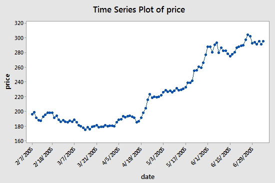
Consecutive values appear to follow one another fairly closely, suggesting an autoregression model could be appropriate. We next look at a plot of partial autocorrelations for the data:
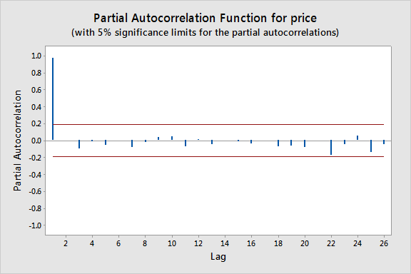
To obtain this in Minitab select Stat > Time Series > Partial Autocorrelation. Here we notice that there is a significant spike at a lag of 1 and much lower spikes for the subsequent lags. Thus, an AR(1) model would likely be feasible for this data set.
Approximate bounds can also be constructed (as given by the red lines in the plot above) for this plot to aid in determining large values. Approximate \((1-\alpha)\times 100\%\) significance bounds are given by \(\pm z_{1-\alpha/2}/\sqrt{n}\). Values lying outside of either of these bounds are indicative of an autoregressive process.
We can next create a lag-1 price variable and consider a scatterplot of price versus this lag-1 variable:
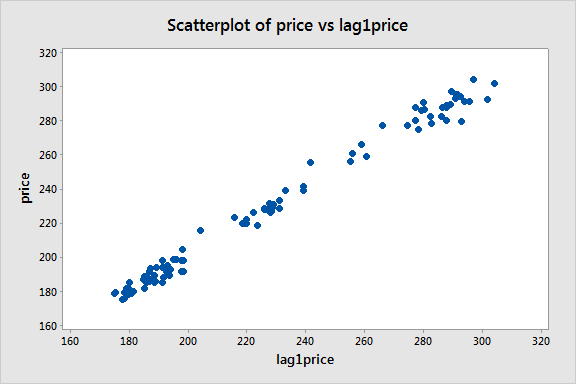
There appears to be a moderate linear pattern, suggesting that the first-order autoregression model
\(\begin{equation*} y_{t}=\beta_{0}+\beta_{1}y_{t-1}+\epsilon_{t} \end{equation*}\)
could be useful.
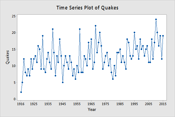
Example 14-2: Quake Data
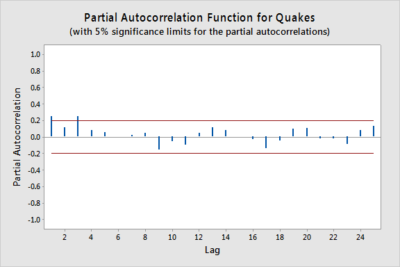
Let \(y_t\) = the annual number of worldwide earthquakes with a magnitude greater than 7 on the Richter scale for n = 100 years (Earthquakes data obtained from the USGS Website). The plot below gives a time series plot for this dataset.
The plot below gives a plot of the PACF (partial autocorrelation function), which can be interpreted to mean that a third-order autoregression may be warranted since there are notable partial autocorrelations for lags 1 and 3.
The next step is to do a multiple linear regression with the number of quakes as the response variable and lag-1, lag-2, and lag-3 quakes as the predictor variables. (In Minitab, we used Stat >> Time Series >> Lag to create the lag variables.) In the results below we see that the lag-3 predictor is significant at the 0.05 level (and the lag-1 predictor p-value is also relatively small).
Model Summary
| S | R-sq | R-sq(adj) | R-sq(pred) |
|---|---|---|---|
| 3.85068 | 13.88% | 11.10% | 6.47% |
Coefficients
| Term | Coef | SE Coef | T-Value | P-Value | VIF |
|---|---|---|---|---|---|
| Constant | 6.45 | 1.79 | 3.61 | 0.000 | |
| lag1Quakes | 0.164 | 0.101 | 1.63 | 0.106 | 1.07 |
| lag2Quakes | 0.071 | 0.101 | 0.70 | 0.484 | 1.12 |
| lag3Quakes | 0.2693 | 0.0978 | 2.75 | 0.007 | 1.09 |
Regression Equation
Quakes = 6.45 + 0.164 lag1Quakes + 0.071 lag2Quakes + 0.2693 lag3Quakes
T.2.2 - Regression with Autoregressive Errors
T.2.2 - Regression with Autoregressive ErrorsNext, let us consider the problem in which we have a y-variable and x-variables all measured as a time series. As an example, we might have y as the monthly accidents on an interstate highway and x as the monthly amount of travel on the interstate, with measurements observed for 120 consecutive months. A multiple (time series) regression model can be written as:
\(\begin{equation} y_{t}=\textbf{X}_{t}\beta+\epsilon_{t}. \end{equation}\)
The difficulty that often arises in this context is that the errors (\(\epsilon_{t}\)) may be correlated with each other. In other words, we have autocorrelation or a dependency between the errors.
We may consider situations in which the error at one specific time is linearly related to the error at the previous time. That is, the errors themselves follow a simple linear regression model that can be written as
\(\begin{equation} \epsilon_{t}=\rho\epsilon_{t-1}+\omega_{t}. \end{equation}\)
Here, \(|\rho|<1 \) is called the autocorrelation parameter, and the \(\omega_{t}\) term is a new error term that follows the usual assumptions that we make about regression errors: \(\omega_{t}\sim_{iid}N(0,\sigma^{2})\). (Here "iid" stands for "independent and identically distributed.) So, this model says that the error at time t is predictable from a fraction of the error at time t - 1 plus some new perturbation \(\omega_{t}\).
Our model for the \(\epsilon_{t}\) errors of the original Y versus X regression is an autoregressive model for the errors, specifically AR(1) in this case. One reason why the errors might have an autoregressive structure is that the Y and X variables at time t may be (and most likely are) related to the Y and X measurements at time t – 1. These relationships are being absorbed into the error term of our multiple linear regression model that only relates Y and X measurements made at concurrent times. Notice that the autoregressive model for the errors is a violation of the assumption that we have independent errors and this creates theoretical difficulties for ordinary least squares estimates of the beta coefficients. There are several different methods for estimating the regression parameters of the Y versus X relationship when we have errors with an autoregressive structure and we will introduce a few of these methods later.
The error terms \(\epsilon_{t}\) still have mean 0 and constant variance:
\(\begin{align*} \mbox{E}(\epsilon_{t})&=0 \\ \mbox{Var}(\epsilon_{t})&=\frac{\sigma^{2}}{1-\rho^{2}}. \end{align*}\)
However, the covariance (a measure of the relationship between two variables) between adjacent error terms is:
\(\begin{equation*} \mbox{Cov}(\epsilon_{t},\epsilon_{t-1})=\rho\biggl(\frac{\sigma^{2}}{1-\rho^{2}}\biggr), \end{equation*}\)
which implies the coefficient of correlation (a unitless measure of the relationship between two variables) between adjacent error terms is:
\(\begin{equation*} \mbox{Corr}(\epsilon_{t},\epsilon_{t-1})=\frac{\mbox{Cov}(\epsilon_{t},\epsilon_{t-1})}{\sqrt{\mbox{Var}(\epsilon_{t})\mbox{Var}(\epsilon_{t-1})}}=\rho, \end{equation*}\)
which is the autocorrelation parameter we introduced above.
We can use partial autocorrelation function (PACF) plots to help us assess appropriate lags for the errors in a regression model with autoregressive errors. Specifically, we first fit a multiple linear regression model to our time series data and store the residuals. Then we can look at a plot of the PACF for the residuals versus the lag. Large sample partial autocorrelations that are significantly different from 0 indicate lagged terms of \(\epsilon\) that may be useful predictors of \(\epsilon_{t}\).
T.2.3 - Testing and Remedial Measures for Autocorrelation
T.2.3 - Testing and Remedial Measures for AutocorrelationHere we present some formal tests and remedial measures for dealing with error autocorrelation.
Durbin-Watson Test
We usually assume that the error terms are independent unless there is a specific reason to think that this is not the case. Usually, violation of this assumption occurs because there is a known temporal component for how the observations were drawn. The easiest way to assess if there is dependency is by producing a scatterplot of the residuals versus the time measurement for that observation (assuming you have the data arranged according to a time sequence order). If the data are independent, then the residuals should look randomly scattered about 0. However, if a noticeable pattern emerges (particularly one that is cyclical) then dependency is likely an issue.
Recall that if we have a first-order autocorrelation with the errors, then the errors are modeled as:
\(\begin{equation*} \epsilon_{t}=\rho\epsilon _{t-1}+\omega_{t}, \end{equation*}\)
where \(|\rho|<1\) and the \(\omega_{t}\sim_{iid}N(0,\sigma^{2})\). If we suspect first-order autocorrelation with the errors, then a formal test does exist regarding the parameter \(\rho\). In particular, the Durbin-Watson test is constructed as:
\(\begin{align*} \nonumber H_{0}&\colon \rho=0 \\ \nonumber H_{A}&\colon \rho\neq 0. \end{align*}\)
So the null hypothesis of \(\rho=0\) means that \(\epsilon_{t}=\omega_{t}\), or that the error term in one period is not correlated with the error term in the previous period, while the alternative hypothesis of \(\rho\neq 0\) means the error term in one period is either positively or negatively correlated with the error term in the previous period. Oftentimes, a researcher will already have an indication of whether the errors are positively or negatively correlated. For example, a regression of oil prices (in dollars per barrel) versus the gas price index will surely have positively correlated errors. When the researcher has an indication of the direction of the correlation, then the Durbin-Watson test also accommodates the one-sided alternatives \(H_{A}\colon\rho< 0\) for negative correlations or \(H_{A}\colon\rho> 0\) for positive correlations (as in the oil example).
The test statistic for the Durbin-Watson test on a data set of size n is given by:
\(\begin{equation*} D=\dfrac{\sum_{t=2}^{n}(e_{t}-e_{t-1})^{2}}{\sum_{t=1}^{n}e_{t}^{2}}, \end{equation*}\)
where \(e_{t}=y_{t}-\hat{y}_{t}\) are the residuals from the ordinary least squares fit. The DW test statistic varies from 0 to 4, with values between 0 and 2 indicating positive autocorrelation, 2 indicating zero autocorrelation, and values between 2 and 4 indicating negative autocorrelation. Exact critical values are difficult to obtain, but tables (for certain significance values) can be used to make a decision (e.g., see the tables on the Durbin Watson Significance Tables, where N represents the sample size, n, and \(\Lambda\) represents the number of regression parameters, p). The tables provide a lower and upper bound, called \(d_{L}\) and \(d_{U}\), respectively. In testing for positive autocorrelation, if \(D<d_{L}\) then reject \(H_{0}\), if \(D>d_{U}\) then fail to reject \(H_{0}\), or if \(d_{L}\leq D\leq d_{U}\), then the test is inconclusive. While the prospect of having an inconclusive test result is less than desirable, there are some programs that use exact and approximate procedures for calculating a p-value. These procedures require certain assumptions about the data which we will not discuss. One "exact" method is based on the beta distribution for obtaining p-values.
To illustrate, consider the Blaisdell Company example from page 489 of Applied Linear Regression Models (4th ed) by Kutner, Nachtsheim, and Neter. If we fit a simple linear regression model with response comsales (company sales in $ millions) and predictor indsales (industry sales in $ millions) and click the "Results" button in the Regression Dialog and check "Durbin-Watson statistic" we obtain the following output:
Coefficients
| Term | Coef | SE Coef | T-Value | P-Value | VIF |
|---|---|---|---|---|---|
| Constant | -1.455 | 0.214 | -6.79 | 0.000 | |
| indsales | 0.17628 | 0.00144 | 122.02 | 0.000 | 1.00 |
Durbin-Watson Statistic = 0.734726
Since the value of the Durbin-Watson Statistic falls below the lower bound at a 0.01 significance level (obtained from a table of Durbin-Watson test bounds), there is strong evidence the error terms are positively correlated.
Ljung-Box Q Test
The Ljung-Box Q test (sometimes called the Portmanteau test) is used to test whether or not observations over time are random and independent. In particular, for a given k, it tests the following:
\(\begin{align*} \nonumber H_{0}&\colon \textrm{the autocorrelations up to lag} \ k \ \textrm{are all 0} \\ \nonumber H_{A}&\colon \textrm{the autocorrelations of one or more lags differ from 0}. \end{align*}\)
The test statistic is calculated as:
\(\begin{equation*} Q_{k}=n(n+2)\sum_{j=1}^{k}\dfrac{{r}^{2}_{j}}{n-j}, \end{equation*}\)
which is approximately \(\chi^{2}_{k}\)-distributed.
To illustrate how the test works for k=1, consider the Blaisdell Company example from above. If we store the residuals from a simple linear regression model with response comsales and predictor indsales and then find the autocorrelation function for the residuals (select Stat > Time Series > Autocorrelation), we obtain the following output:
Autocorrelation Function: RESI1
| Lag | ACF | T | LBQ |
|---|---|---|---|
| 1 | 0.624005 | 2.80 | 9.08 |
The Ljung-Box Q test statistic of 9.08 corresponds to a \(\chi^{2}_{1}\) p-value of 0.0026, so there is strong evidence the lag-1 autocorrelation is non-zero.
Remedial Measures
When autocorrelated error terms are found to be present, then one of the first remedial measures should be to investigate the omission of a key predictor variable. If such a predictor does not aid in reducing/eliminating autocorrelation of the error terms, then certain transformations on the variables can be performed. We discuss three transformations that are designed for AR(1) errors. Methods for dealing with errors from an AR(k) process do exist in the literature but are much more technical in nature.
Cochrane-Orcutt Procedure
The first of the three transformation methods we discuss is called the Cochrane-Orcutt procedure, which involves an iterative process (after identifying the need for an AR(1) process):
Estimate \(\rho\) for \(\begin{equation*} \epsilon_{t}=\rho\epsilon_{t-1}+\omega_{t} \end{equation*}\) by performing a regression through the origin. Call this estimate r.
Transform the variables from the multiple regression model \(\begin{equation*} y_{t}=\beta_{0}+\beta_{1}x_{t,1}+\ldots+\beta_{p-1}x_{t,p-1}+\epsilon_{t} \end{equation*}\) by setting \(y_{t}^{*}=y_{t}-ry_{t-1}\) and \(x_{t,j}^{*}=x_{t,j}-rx_{t-1,j}\) for \(j=1,\ldots,p-1\).
Regress \(y_{t}^{*}\) on the transformed predictors using ordinary least squares to obtain estimates \(\hat{\beta}_{0}^{*},\ldots,\hat{\beta}_{p-1}^{*}\). Look at the error terms for this fit and determine if autocorrelation is still present (such as using the Durbin-Watson test). If autocorrelation is still present, then iterate this procedure. If it appears to be corrected, then transform the estimates back to their original scale by setting \(\hat{\beta}_{0}=\hat{\beta}_{0}^{*}/(1-r)\) and \(\hat{\beta}_{j}=\hat{\beta}_{j}^{*}\) for \(j=1,\ldots,p-1\). Notice that only the intercept parameter requires a transformation. Furthermore, the standard errors of the regression estimates for the original scale can also be obtained by setting \(\textrm{s.e.}(\hat{\beta}_{0})=\textrm{s.e.}(\hat{\beta}_{0}^{*})/(1-r)\) and \(\textrm{s.e.}(\hat{\beta}_{j})=\textrm{s.e.}(\hat{\beta}_{j}^{*})\) for \(j=1,\ldots,p-1\).
To illustrate the Cochrane-Orcutt procedure, consider the Blaisdell Company example from above:
- Store the residuals, RESI1, from a simple linear regression model with response comsales and predictor indsales.
- Use Minitab's Calculator to define a lagged residual variable, lagRESI1 = LAG(RESI1,1).
- Fit a simple linear regression model with response RESI1 and predictor lagRESI1 and no intercept. Use the Storage button to store the Coefficients. We find the estimated slope from this regression to be 0.631164, which is the estimate of the autocorrelation parameter, \(\rho\).
- Use Minitab's Calculator to define a transformed response variable, Y_co = comsales-0.631164*LAG(comsales,1).
- Use Minitab's Calculator to define a transformed predictor variable, X_co = indsales-0.631164*LAG(indsales,1).
- Fit a simple linear regression model with response Y_co and predictor X_co to obtain the following output:
Coefficients
| Term | Coef | SE Coef | T-Value | P-Value | VIF |
|---|---|---|---|---|---|
| Constant | -0.394 | 0.167 | -2.36 | 0.031 | |
| X_co | 0.17376 | 0.00296 | 58.77 | 0.000 | 1.00 |
Durbin-Watson Statistic = 1.65025
- Since the value of the Durbin-Watson Statistic falls above the upper bound at a 0.01 significance level (obtained from a table of Durbin-Watson test bounds), there is no evidence the error terms are positively correlated in the model with the transformed variables.
- Transform the intercept parameter, -0.394/(1-0.631164) = -1.068, and its standard error, 0.167/(1-0.631164) = 0.453 (the slope estimate and standard error don't require transformation).
- The fitted regression function for the original variables is predicted comsales = -1.068 + 0.17376 indsales.
One thing to note about the Cochrane-Orcutt approach is that it does not always work properly. This occurs primarily because if the errors are positively autocorrelated, then r tends to underestimate \(\rho\). When this bias is serious, then it can seriously reduce the effectiveness of the Cochrane-Orcutt procedure.
Hildreth-Lu Procedure
The Hildreth-Lu procedure is a more direct method for estimating \(\rho\). After establishing that the errors have an AR(1) structure, follow these steps:
- Select a series of candidate values for \(\rho\) (presumably values that would make sense after you assessed the pattern of the errors).
- For each candidate value, regress \(y_{t}^{*}\) on the transformed predictors using the transformations established in the Cochrane-Orcutt procedure. Retain the SSEs for each of these regressions.
- Select the value which minimizes the SSE as an estimate of \(\rho\).
Notice that this procedure is similar to the Box-Cox transformation discussed previously and that it is not iterative like the Cochrane-Orcutt procedure.
To illustrate the Hildreth-Lu procedure, consider the Blaisdell Company example from above:
- Use Minitab's Calculator to define a transformed response variable, Y_hl.1 = comsales-0.1*LAG(comsales,1).
- Use Minitab's Calculator to define a transformed predictor variable, X_hl.1 = indsales-0.1*LAG(indsales,1).
- Fit a simple linear regression model with response Y_hl.1 and predictor X_hl.1 and record the SSE.
- Repeat steps 1-3 for a series of estimates of \(\rho\) to find when SSE is minimized (0.96 leads to the minimum in this case).
- The output for this model is:
Analysis of Variances
| Source | DF | Adj SS | Adj Ms | F-Value | P-Value |
|---|---|---|---|---|---|
| Regression | 1 | 2.31988 | 2.31988 | 550.26 | 0.000 |
| X_h1.96 | 1 | 2.31988 | 2.31988 | 550.26 | 0.000 |
| Error | 17 | 0.07167 | 0.00422 | ||
| Total | 18 | 2.39155 |
Coefficients
| Term | Coef | SE Coef | T-Value | P-Value | VIF |
|---|---|---|---|---|---|
| Constant | 0.0712 | 0.0580 | 1.23 | 0.236 | |
| X_h1.96 | 0.16045 | 0.00684 | 23.46 | 0.000 | 1.00 |
Durbin-Watson Statistic = 1.72544
- Since the value of the Durbin-Watson Statistic falls above the upper bound at a 0.01 significance level (obtained from a table of Durbin-Watson test bounds), there is no evidence the error terms are positively correlated in the model with the transformed variables.
- Transform the intercept parameter, 0.0712/(1-0.96) = 1.78, and its standard error, 0.0580/(1-0.96) = 1.45 (the slope estimate and standard error don't require transforming).
- The fitted regression function for the original variables is predicted comsales = 1.78 + 0.16045 indsales.
First Differences Procedure
Since \(\rho\) is frequently large for AR(1) errors (especially in economics data), many have suggested just setting \(\rho\) = 1 in the transformed model of the previous two procedures. This procedure is called the first differences procedure and simply regresses \(y_{t}^{*}=y_{t}-y_{t-1}\) on the \(x_{t,j}^{*}=x_{t,j}-x_{t-1,j}\) for \(j=1,\ldots,p-1\) using regression through the origin. The estimates from this regression are then transformed back, setting \(\hat{\beta}_{j}=\hat{\beta}_{j}^{*}\) for \(j=1,\ldots,p-1 \) and \(\hat{\beta}_{0}=\bar{y}-(\hat{\beta}_{1}\bar{x}_{1}+\ldots+\hat{\beta}_{p-1}\bar{x}_{p-1})\).
To illustrate the first differences procedure, consider the Blaisdell Company example from above:
- Use Minitab's Calculator to define a transformed response variable, Y_fd = comsales-LAG(comsales,1).
- Use Minitab's Calculator to define a transformed predictor variable, X_fd = indsales-LAG(indsales,1).
- Fit a simple linear regression model with response Y_fd and predictor X_fd and use the "Results" button to select the Durbin-Watson statistic: Durbin-Watson Statistic = 1.74883
- Since the value of the Durbin-Watson Statistic falls above the upper bound at a 0.01 significance level (obtained from a table of Durbin-Watson test bounds), there is no evidence the error terms are correlated in the model with the transformed variables.
- Fit a simple linear regression model with response Y_fd and predictor X_fd and no intercept. The output for this model is:
Coefficients
| Term | Coef | SE Coef | T-Value | P-Value | VIF |
|---|---|---|---|---|---|
| X_fd | 0.16849 | 0.00510 | 33.06 | 0.000 | 1.00 |
- Find the sample mean of comsales and indsales using Stat > Basic Statistics > Display Descriptive Statistics:
| Variable | N | N* | Mean | SE Mean | StDev | Minimum | Q1 | Median | Q3 | Maximum |
|---|---|---|---|---|---|---|---|---|---|---|
| comsales | 20 | 0 | 24.569 | 0.539 | 2.410 | 20.960 | 22.483 | 24.200 | 26.825 | 28.970 |
| indsales | 20 | 0 | 147.62 | 3.06 | 13.67 | 127.30 | 135.53 | 145.95 | 159.85 | 171.70 |
- Calculate the estimated intercept parameter, \(\hat \beta_0 = 24.569 - 0.16849(147.62) = - 0.303\).
- The fitted regression function for the original variables is predicted comsales = -0.303 + 0.16849 indsales.
Forecasting Issues
When calculating forecasts for regression with autoregressive errors, it is important to utilize the modeled error structure as part of our process. For example, for AR(1) errors, \(\epsilon_{t}=\rho\epsilon_{t-1}+\omega_{t}\), our fitted regression equation is
\(\begin{equation*} \hat{y}_{t}=b_{0}+b_{1}x_{t}, \end{equation*}\)
with forecasts of \(y\) at time \(t\), denoted \(F_{t}\), computed as:
\(\begin{equation*} F_{t}=\hat{y}_{t}+e_{t}=\hat{y}_{t}+re_{t-1}. \end{equation*}\)
So, we can compute forecasts of \(y\) at time \(t+1\), denoted \(F_{t+1}\), iteratively:
- Compute the fitted value for time period t, \(\hat{y}_{t}=b_{0}+b_{1}x_{t}\)
- Compute the residual for time period t, \(e_{t}=y_{t}-\hat{y}_{t}\).
- Compute the fitted value for time period t+1, \(\hat{y}_{t+1}=b_{0}+b_{1}x_{t+1}\).
- Compute the forecast for time period t+1, \(F_{t+1}=\hat{y}_{t+1}+re_{t}\).
- Iterate.
To illustrate forecasting for the Cochrane-Orcutt procedure, consider the Blaisdell Company example from above. Suppose we wish to forecast comsales for time period 21 when indsales are projected to be $175.3 million:
- The fitted value for time period 20 is \(\hat{y}_{20} = -1.068+0.17376(171.7)) = 28.767\).
- The residual for time period 20 is \(e_{20} = y_{20}-\hat{y}_{20} = 28.78 - 28.767 = 0.013\).
- The fitted value for time period 21, \(\hat{y}_{21} = -1.068+0.17376(175.3)) = 29.392\).
- The forecast for time period 21 is \(F_{21}=29.392+0.631164(0.013)=29.40\).
Note that this procedure is not needed when simply using the lagged response variable as a predictor, e.g., in the first-order autoregression model
\(\begin{equation*} y_{t}=\beta_{0}+\beta_{1}y_{t-1}+\epsilon_{t} \end{equation*}.\)
T.2.4 - Examples of Applying Cochrane-Orcutt Procedure
T.2.4 - Examples of Applying Cochrane-Orcutt ProcedureExample 14-3: Employee Data

The next data set gives the number of employees (in thousands) for a metal fabricator and one of their primary vendors for each month over a 5-year period, so n = 60 (Employee data). A simple linear regression analysis was implemented:
\(\begin{equation*} y_{t}=\beta_{0}+\beta_{1}x_{t}+\epsilon_{t}, \end{equation*}\)
where \(y_{t}\) and \(x_{t}\) are the number of employees during time period t at the metal fabricator and vendor, respectively.
A plot of the number of employees at the fabricator versus the number of employees at the vendor with the ordinary least squares regression line overlaid is given below in plot (a). A scatterplot of the residuals versus t (the time ordering) is given in plot (b).
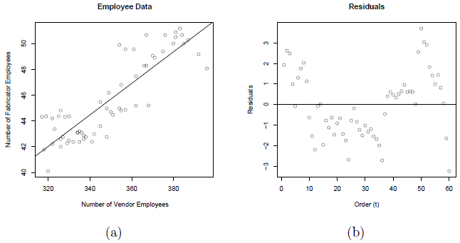
Notice the non-random trend suggestive of autocorrelated errors in the scatterplot. The estimated equation is \(y_{t}=2.85+0.12244x_{t}\), which is given in the following summary output:
Model Summary
| S | R-sq | R-sq(adj) | R-sq(pred) |
|---|---|---|---|
| 1.58979 | 74.43% | 73.99% | 72.54% |
Coefficients
| Term | Coef | SE Coef | T-Value | P-Value | VIF |
|---|---|---|---|---|---|
| Constant | 2.85 | 3.30 | 0.86 | 0.392 | |
| vendor | 0.12244 | 0.00942 | 12.99 | 0.000 | 1.00 |
Regression Equation
metal = 2.85 + 0.12244 vendor
The plot below gives the PACF plot of the residuals, which helps us decide the lag values. (Minitab: Store the residuals from the regression model fit then select Stat > Time Series > Partial Autocorrelation and use the stored residuals as the "Series.")
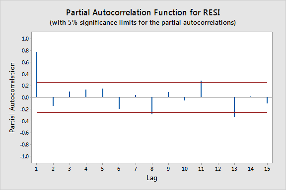
In particular, it looks like there is a lag of 1 since the lag-1 partial autocorrelation is so large and way beyond the "5% significance limits" shown by the red lines. (The partial autocorrelations at lags 8, 11, and 13 are only slightly beyond the limits and would lead to an overly complex model at this stage of the analysis.) We can also obtain the output from the Durbin-Watson test for serial correlation (Minitab: click the "Results" button in the Regression Dialog and check "Durbin-Watson statistic."):
Durbin-Watson Statistic
Durbin-Watson Statistic = 0.359240
To find the p-value for this test statistic we need to look up a Durbin-Watson critical values table, which in this case indicates a highly significant p-value of approximately 0. (In general Durbin-Watson statistics close to 0 suggest significant positive autocorrelation.) A lag of 1 appears appropriate.
Since we decide upon using AR(1) errors, we will have to use one of the procedures we discussed earlier. In particular, we will use the Cochrane-Orcutt procedure. Start by fitting a simple linear regression model with a response variable equal to the residuals from the model above and a predictor variable equal to the lag-1 residuals and no intercept to obtain the slope estimate, r = 0.831385.
Now, transform to \(y_{t}^{*}=y_{t}-ry_{t-1}\) and \(x_{t}^{*}=x_{t}-rx_{t-1}\). Perform a simple linear regression of \(y_{t}^{*}\) on \(x_{t}^{*}\). The resulting regression estimates from the Cochrane-Orcutt procedure are:
\(\begin{align*} \hat{\beta}_{1}^{*}&=0.0479=\hat{\beta}_{1} \\ \hat{\beta}_{0}^{*}&=4.876\Rightarrow\hat{\beta}_{0}=\frac{4.876}{1-0.831385}=28.918. \end{align*}\)
The corresponding standard errors are:
\(\begin{align*} \mbox{s.e.}(\hat{\beta}_{1}^{*})&=0.0130=\mbox{s.e.}(\hat{\beta}_{1})\\ \mbox{s.e.}(\hat{\beta}_{0}^{*})&=0.787\Rightarrow\mbox{s.e.}(\hat{\beta}_{0})=\frac{0.787}{1-0.831385}=4.667. \end{align*}\)
Notice that the correct standard errors (from the Cochrane-Orcutt procedure) are larger than the incorrect values from the simple linear regression on the original data. If ordinary least squares estimation is used when the errors are autocorrelated, the standard errors often are underestimated. It is also important to note that this does not always happen. Underestimation of the standard errors is an "on average" tendency overall problem.
Example 14-4: Oil Data
The data are from U.S. oil and gas price index values for 82 months (dataset no longer available). There is a strong linear pattern for the relationship between the two variables, as can be seen below.
We start the analysis by doing a simple linear regression. Minitab results for this analysis are given below.
Coefficients
| Predictor | Coef | SE Coef | T-Value | P-Value |
|---|---|---|---|---|
| Constant | -31.349 | 5.219 | -6.01 | 0.000 |
| Oil | 1.17677 | 0.02305 | 51.05 | 0.000 |
Regression Equation
Gas = -31.3 + 1.18 Oil
The residuals in time order show a dependent pattern (see the plot below).
The slow cyclical pattern that we see happens because there is a tendency for residuals to keep the same algebraic sign for several consecutive months. We also used Stat >> Time Series >> Lag to create a column of the lag 1 residuals. The correlation coefficient between the residuals and the lagged residuals is calculated to be 0.829 (and is calculated using Stat >> Basic Stats >> Correlation, which can be seen at the bottom of the figure above).
So, the overall analysis strategy in presence of autocorrelated errors is as follows:
- Do an ordinary regression. Identify the difficulty in the model (autocorrelated errors).
- Using the stored residuals from the linear regression, use regression to estimate the model for the errors, \(\epsilon_t = \rho\epsilon_{t-1} + u_t\) where the \(u_t\) are iid with mean 0 and variance \(\sigma^{2}\).
- Adjust the parameter estimates and their standard errors from the original regression.
A Method for Adjusting the Original Parameter Estimates (Cochrane-Orcutt Method)
- Let \(\hat{\rho}\) = estimated lag 1 autocorrelation in the residuals from the ordinary regression (in the U.S. oil example, \(\hat{\rho} = 0.829\)).
- Let \({y^{*}}_t = y_t − \hat{\rho} y_{t-1}\). This will be used as a response variable.
- Let \({x^{*}}_t = x_t − \hat{\rho} x_{t-1}\). This will be used as a predictor variable.
- Do an “ordinary” regression between \({y^*}_t\) and \({x^*}_t\) . This model should have time-independent residuals.
- The sample slope from the regression directly estimates \(\beta_1\), the slope of the relationship between the original y and x.
- The correct estimate of the intercept for the original model y versus x relationship is calculated as \(\beta_0=\hat{\beta}_0^* / (1-\hat{\rho})\), where \(\hat{\beta}_0\) is the sample intercept obtained from the regression done with the modified variables.
Returning to the U.S. oil data, the value of \(\hat{\rho} = 0.829\) and the modified variables are \(\mathbf{ynew} = y_t − 0.829 y_{t-1}\) and \(\mathbf{xnew} = x_t −0.829 x_{t-1}\). The regression results are given below.
Coefficients
| Predictor | Coef | SE Coef | T | P |
|---|---|---|---|---|
| Constant | -1.412 | 2.529 | -0.56 | 0.578 |
| xnew | 1.08073 | 0.05960 | 18.13 | 0.000 |
Parameter Estimates for the Original Model
Our real goal is to estimate the original model \(y_t = \beta_0 +\beta_1 x_t + \epsilon_t\) . The estimates come from the results just given.
\(\hat{\beta}_1=1.08073\)
\(\hat{\beta}_0=\dfrac{-1.412}{1-0.829}=-8.2573\)
These estimates give the sample regression model:
\(y_t = −8.257 + 1.08073 x_t + \epsilon_t\)
with \(\epsilon_t = 0.829 \epsilon_{t-1} + u_t\) , where \(u_t\)’s are iid with mean 0 and variance \(\sigma^{2}\).
Correct Standard Errors for the Coefficients
- The correct standard error for the slope is taken directly from the regression with the modified variables.
- The correct standard error for the intercept is \(\text{s.e.}\hat{\beta}_0=\dfrac{\text{s.e.}\hat{\beta}_0^*}{1-\hat{\rho}}\).
Correct and incorrect estimates for the coefficients:
| Coefficient | Correct Estimate | Correct Standard Error |
|---|---|---|
| Intercept | −1.412 / (1−0.829) = −8.2573 | 2.529 / (1−0.829) = 14.79 |
| Slope | 1.08073 | 0.05960 |
| Incorrect Estimate | Incorrect Standard Error | |
| Intercept | -31.349 | 5.219 |
| Slope | 1.17677 | 0.02305 |
This table compares the correct standard errors to the incorrect estimates based on the ordinary regression. The “correct” estimates come from the work done in this section of the notes. The incorrect estimates are from the original regression estimates reported above. Notice that the correct standard errors are larger than the incorrect values here. If ordinary least squares estimation is used when the errors are autocorrelated, the standard errors often are underestimated. It is also important to note that this does not always happen. Overestimation of the standard errors is an “on average” tendency overall problem.
Forecasting Issues
When calculating forecasts for time series, it is important to utilize \(\epsilon_t = \rho \epsilon_{t-1} + u_t\) as part of the process. In the U.S. oil example,
\(F_t=\hat{y}_t + e_t = −8.257 + 1.08073 x_t + e_t = −8.257 + 1.08073 x_t + 0.829 e_{t-1}\)
Values of \(F_t\) are computed iteratively:
- Compute \(\hat{y}_1= −8.257 + 1.08073x_1\) and \(e_1=y_1-\hat{y}_1\).
- Compute \(\hat{y}_2= −8.257 + 1.08073x_2\) and use the value of \(e_1\) when computing \(F_2 = \hat{y}_2 + 0.829e_1\).
- Determine \(e_2=y_2-\hat{y}_2\).
- Compute \(\hat{y}_3= −8.257 + 1.08073x_3\) and use the value of \(e_2\) when computing \(F_3 = \hat{y}_3 + 0.829e_2\).
- Iterate.
T.2.5 - Advanced Methods
T.2.5 - Advanced MethodsThis section provides a few more advanced techniques used in time series analysis. While they are more peripheral to the autoregressive error structures that we have discussed, they are germane to this lesson since these models are constructed in a regression framework. Moreover, a course in regression is generally a prerequisite for any time series course, so it is helpful to at least provide exposure to some of the more commonly studied time series techniques.
T.2.5.1 - ARIMA Models
T.2.5.1 - ARIMA ModelsSince many of the time series models have a regression structure, it is beneficial to introduce a general class of time series models called autoregressive integrated moving averages or ARIMA models. They are also referred to as Box-Jenkins models, due to the systematic methodology of identifying, fitting, checking, and utilizing ARIMA models, which was popularized by George Box and Gwilym Jenkins in 1976. Before we write down a general ARIMA model, we need to introduce a few additional concepts.
Suppose we have the time series \(Y_{1},Y_{2},\ldots,Y_{t}\). If the value for each Y is determined exactly by a mathematical formula, then the series is said to be deterministic. If the future values of Y can only be described through their probability distribution, then the series is said to be a stochastic process.1 A special class of stochastic processes is a stationary stochastic process, which occurs when the probability distribution for the process is the same for all starting values of t. Such a process is completely defined by its mean, variance, and autocorrelation function. When a time series exhibits nonstationary behavior, then part of our objective will be to transform it into a stationary process.
When stationarity is not an issue, then we can define an autoregressive moving average or ARMA model as follows:
\(\begin{equation*} Y_{t}=\sum_{i=1}^{p}\phi_{i}Y_{t-i}+a_{t}-\sum_{j=1}^{q}\theta_{j}a_{t-j}, \end{equation*} \)
where \(\phi_{1},\ldots,\phi_{p}\) are the autoregressive parameters to be estimated, \(\theta_{1},\ldots,\theta_{q}\) are the moving average parameters to be estimated, and \(a_{1},\ldots,a_{t}\) are a series of unknown random errors (or residuals) that are assumed to follow a normal distribution. This is also referred to as an ARMA(p,q) model. The model can be simplified by introducing the Box-Jenkins backshift operator, which is defined by the following relationship:
\(\begin{equation*} B^{p}X_{t}=X_{t-p}, \end{equation*}\)
such that \(X_{1},\ldots,X_{t}\) is any time series and \(p<t\). Using the backshift notation yields the following:
\(\begin{equation*} \biggl(1-\sum_{i=1}^{p}\phi_{i}B^{i}\biggr)Y_{t}=\biggl(1-\sum_{j=1}^{q}\theta_{j}B^{j}\biggr)a_{t}, \end{equation*}\)
which is often reduced further to
\(\begin{equation*} \phi_{p}(B)Y_{t}=\theta_{q}(B)a_{t}, \end{equation*}\)
where \(\phi_{p}(B)=(1-\sum_{i=1}^{p}\phi_{i}B^{i})\) and \(\theta_{q}(B)=(1-\sum_{j=1}^{q}\theta_{j}B^{j})\).
When time series exhibit nonstationary behavior (which commonly occurs in practice), then the ARMA model presented above can be extended and written using differences, which are defined as follows:
\(\begin{align*} W_{t}&=Y_{t}-Y_{t-1}=(1-B)Y_{t}\\ W_{t}-W_{t-1}&=Y_{t}-2Y_{t-1}+Y_{t-2}\\ &=(1-B)^{2}Y_{t}\\ & \ \ \vdots\\ W_{t}-\sum_{k=1}^{d}W_{t-k}&=(1-B)^{d}Y_{t}, \end{align*}\)
where d is the order of differencing. Replacing \(Y_{t}\) in the ARMA model with the differences defined above yields the formal ARIMA(p,d,q) model:
\(\begin{equation*} \phi_{p}(B)(1-B)^{d}Y_{t}=\theta_{q}(B)a_{t}. \end{equation*}\)
An alternative way to deal with nonstationary behavior is to simply fit a linear trend to the time series and then fit a Box-Jenkins model to the residuals from the linear fit. This will provide a different fit and a different interpretation, but is still a valid way to approach a process exhibiting nonstationarity.
Seasonal time series can also be incorporated into a Box-Jenkins framework. The following general model is usually recommended:
\(\begin{equation*} \phi_{p}(B)\Phi(P)(B^{s})(1-B)^{d}(1-B^{s})^{D}Y_{t}=\theta_{q}(B)\Theta_{Q}(B^{s})a_{t}, \end{equation*}\)
where p, d, and q are as defined earlier, s is a (known) number of seasons per timeframe (e.g., years), D is the order of the seasonal differencing, and P and Q are the autoregressive and moving average orders, respectively, when accounting for the seasonal shift. Moreover, the operator polynomials \(\phi_{p}(B)\) and \(\theta_{q}(B)\) are as defined earlier, while \(\Phi_{P}(B)=(1-\sum_{i=1}^{P}\Phi_{i}B^{s\times i})\) and \(\Theta_{Q}(B)=(1-\sum_{j=1}^{Q}\Theta_{j}B^{s\times j})\). Luckily, the maximum value of p, d, q, P, D, and Q is usually 2, so the resulting expression is relatively simple.
With all of the modeling discussion provided above, we will now provide a brief overview of how to implement the Box-Jenkins methodology in practice, which (fortunately) most statistical software packages will perform for you:
- Model Identification: Using plots of the data, autocorrelations, partial autocorrelations, and other information, a class of simple ARIMA models is selected. This amounts to estimating (or guesstimating) an appropriate value for d followed by estimates for p and q (as well as P, D, and Q in the seasonal time series setting).
- Model Estimation: The autoregressive and moving average parameters are found via an optimization method like maximum likelihood.
- Diagnostic Checking: The fitted model is checked for inadequacies by studying the autocorrelations of the residual series (i.e., the time-ordered residuals).
The above is then iterated until there appears to be minimal to no improvement in the fitted model.
1 It should be noted that stochastic processes are itself a heavily-studied and very important statistical subject.
T.2.5.4 - Generalized Least Squares
T.2.5.4 - Generalized Least SquaresWeighted least squares can also be used to reduce autocorrelation by choosing an appropriate weighting matrix. In fact, the method used is more general than weighted least squares. The method of weighted least squares uses a diagonal matrix to help correct for non-constant variance. However, in a model with correlated errors, the errors have a more complicated variance-covariance structure (such as \(\Sigma(1)\) given earlier for the AR(1) model). Thus the weighting matrix for the more complicated variance-covariance structure is non-diagonal and utilizes the method of generalized least squares, of which weighted least squares is a special case. In particular, when \(\mbox{Var}(\textbf{Y})=\mbox{Var}(\pmb{\epsilon})=\Omega\), the objective is to find a matrix \(\Lambda\) such that:
\(\begin{equation*} \mbox{Var}(\Lambda\textbf{Y})=\Lambda\Omega\Lambda^{\textrm{T}}=\sigma^{2}\textbf{I}_{n\times n}, \end{equation*}\)
The generalized least squares estimator (sometimes called the Aitken estimator) takes \(s \Lambda=\sigma\Omega^{1/2}\) and is given by
\(\begin{align*} \hat{\beta}_{\textrm{GLS}}&=\arg\min_{\beta}\|\Lambda(\textbf{Y}-\textbf{X}\beta)\|^{2} \\ &=(\textbf{X}^{\textrm{T}}\Omega^{-1}\textbf{X})^{-1}\textbf{X}^{\textrm{T}}\Omega\textbf{Y}. \end{align*}\)
There is no optimal way of choosing such a weighting matrix \(\Omega\). \(\Omega\) contains \(n(n+1)/2\) parameters, which are too many parameters to estimate, so restrictions must be imposed. The estimate will heavily depend on these assumed restrictions and thus makes the method of generalized least squares difficult to use unless you are savvy (and lucky) enough to choose helpful restrictions.
T.2.5.2 - Exponential Smoothing
T.2.5.2 - Exponential SmoothingThe techniques of the previous section can all be used in the context of forecasting, which is the art of modeling patterns in the data that are usually visible in time series plots and then extrapolated into the future. In this section, we discuss exponential smoothing methods that rely on smoothing parameters, which are parameters that determine how fast the weights of the series decay. For each of the three methods we discuss below, the smoothing constants are found objectively by selecting those values which minimize one of the three error-size criteria below:
\[\begin{align*} \textrm{MSE}&=\frac{1}{n}\sum_{t=1}^{n}e_{t}^{2}\\ \textrm{MAE}&=\frac{1}{n}\sum_{t=1}^{n}|e_{t}|\\ \textrm{MAPE}&=\frac{100}{n}\sum_{t=1}^{n}\biggl|\frac{e_{t}}{Y_{t}}\biggr|, \end{align*}\]
where the error is the difference between the actual value of the time series at time t and the fitted value at time t, which is determined by the smoothing method employed. Moreover, MSE is (as usual) the mean square error, MAE is the mean absolute error, and MAPE is the mean absolute percent error.
Exponential smoothing methods also require initialization since the forecast for period one requires the forecast at period zero, which we do not (by definition) have. Several methods have been proposed for generating starting values. The most commonly used is the backcasting method, which entails reversing the series so that we forecast into the past instead of into the future. This produces the required starting value. Once we have done this, we then switch the series back and apply the exponential smoothing algorithm in a regular manner.
Single exponential smoothing smoothes the data when no trend or seasonal components are present. The equation for this method is:
\[\begin{equation*} \hat{Y}_{t}=\alpha(Y_{t}+\sum_{i=1}^{r}(1-\alpha)^{i}Y_{t-i}), \end{equation*}\]
where \(\hat{Y}_{t}\) is the forecasted value of the series at time t and \(\alpha\) is the smoothing constant. Note that \(r<t\), but r does not have to equal \(t-1\). From the above equation, we see that the method constructs a weighted average of the observations. The weight of each observation decreases exponentially as we move back in time. Hence, since the weights decrease exponentially and averaging is a form of smoothing, the technique was named exponential smoothing. An equivalent ARIMA(0,1,1) model can be constructed to represent the single exponential smoother.
Double exponential smoothing (also called Holt's method) smoothes the data when a trend is present. The double exponential smoothing equations are:
\[\begin{align*} L_{t}&=\alpha Y_{t}+(1-\alpha)(L_{t-1}+T_{t-1})\\ T_{t}&=\beta(L_{t}-L_{t-1})+(1-\beta)T_{t-1}\\ \hat{Y}_{t}&=L_{t-1}+T_{t-1}, \end{align*}\]
where \(L_{t}\) is the level at time t, \(\alpha\) is the weight (or smoothing constant) for the level, \(T_{t}\) is the trend at time t, \(\beta\) is the weight (or smoothing constant) for the trend, and all other quantities are defined as earlier. An equivalent ARIMA(0,2,2) model can be constructed to represent the double exponential smoother.
Finally, Holt-Winters exponential smoothing smoothes the data when trend and seasonality are present; however, these two components can be either additive or multiplicative. For the additive model, the equations are:
\[\begin{align*} L_{t}&=\alpha(Y_{t}-S_{t-p})+(1-\alpha)(L_{t-1}+T_{t-1})\\ T_{t}&=\beta(L_{t}-L_{t-1})+(1-\beta)T_{t-1}\\ S_{t}&=\delta(Y_{t}-L_{t})+(1-\delta)S_{t-p}\\ \hat{Y}_{t}&=L_{t-1}+T_{t-1}+S_{t-p}. \end{align*}\]
For the multiplicative model, the equations are:
\[\begin{align*} L_{t}&=\alpha(Y_{t}/S_{t-p})+(1-\alpha)(L_{t-1}+T_{t-1})\\ T_{t}&=\beta(L_{t}-L_{t-1})+(1-\beta)T_{t-1}\\ S_{t}&=\delta(Y_{t}/L_{t})+(1-\delta)S_{t-p}\\ \hat{Y}_{t}&=(L_{t-1}+T_{t-1})S_{t-p}. \end{align*}\]
For both sets of equations, all quantities are the same as they were defined in the previous models, except now we also have that \(S_{t}\) is the seasonal component at time t, \(\delta\) is the weight (or smoothing constant) for the seasonal component, and p is the seasonal period.
T.2.5.3 - Spectral Analysis
T.2.5.3 - Spectral AnalysisSuppose we believe that a time series, \(Y_{t}\), contains a periodic (cyclic) component. Spectral analysis takes the approach of specifying a time series as a function of trigonometric components. A natural model of the periodic component would be
\(\begin{equation*} Y_{t}=R\cos(ft+d)+e_{t}, \end{equation*}\)
where R is the amplitude of the variation, f is the frequency of periodic variation1, and d is the phase. Using the trigonometric identity \(\cos(A+B)=\cos(A)cos(B)-sin(A)sin(B)\), we can rewrite the above model as
\(\begin{equation*} Y_{t}=a\cos(ft)+b\sin(ft)+e_{t}, \end{equation*}\)
where \(a=R\cos(d)\) and \(b=-R\sin(d)\). Thus, the above is a multiple regression model with two predictors.
Variation in time series may be modeled as the sum of several different individual waves occurring at different frequencies. The generalization of the above model as a sum of k frequencies is
\(\begin{equation*} Y_{t}=\sum_{j=1}^{k}R_{j}\cos(f_{j}t+d_{j})+e_{t}, \end{equation*}\)
which can be rewritten as
\(\begin{equation*} Y_{t}=\sum_{j=1}^{k}a_{j}\cos(f_{j}t)+\sum_{j=1}^{k}b_{j}\sin(f_{j}t)+e_{t}. \end{equation*}\)
Note that if the \(f_{j}\) values were known constants and we let \(X_{t,r}=\cos(f_{r}t)\) and \(Z_{t,r}=\sin(f_{r}t)\), then the above could be rewritten as the multiple regression model
\(\begin{equation*} Y_{t}=\sum_{j=1}^{k}a_{j}X_{t,j}+\sum_{j=1}^{k}b_{j}Z_{t,j}+e_{t}. \end{equation*}\)
The above is an example of a harmonic regression.
Fourier analysis is the study of approximating functions using the sum of sine and cosine terms. Such a sum is called the Fourier series representation of the function. Spectral analysis is identical to Fourier analysis, except that instead of approximating a function, the sum of sine and cosine terms approximates a time series that includes a random component. Moreover, the coefficients in the harmonic regression (i.e., the a's and b's) may be estimated using multiple regression techniques.
Figures can also be constructed to help in the spectral analysis of a time series. While we do not develop the details here, the basic methodology consists of partitioning the total sum of squares into quantities associated with each frequency (like an ANOVA). From these quantities, histograms of the frequency (or wavelength) can be constructed, which are called periodograms. A smoothed version of the periodogram, called a spectral density, can also be constructed and is generally preferred to the periodogram.
Software Help: Time & Series Autocorrelation
Software Help: Time & Series Autocorrelation
The next two pages cover the Minitab and R commands for the procedures in this lesson.
Below is a zip file that contains all the data sets used in this help section:
- employee.txt
- google_stock.txt
- blaisdell.txt
- earthquakes.txt
Minitab Help: Time Series & Autocorrelation
Minitab Help: Time Series & AutocorrelationMinitab®
Google stock (autoregression model)
- Select Stat > Time Series > Time Series Plot, select "price" for the Series, click the Time/Scale button, click "Stamp" under "Time Scale" and select "date" to be a Stamp column.
- Select Stat > Time Series > Partial Autocorrelation to create a plot of partial autocorrelations of price.
- Select Calc > Calculator to calculate a lag-1 price variable.
- Create a basic scatterplot of price vs lag1price.
- Perform a linear regression analysis of price vs lag1price (a first-order autoregression model).
Earthquakes (autoregression model)
- Select Stat > Time Series > Time Series Plot, select "Quakes" for the Series, click the Time/Scale button, click "Stamp" under "Time Scale" and select "Year" to be a Stamp column.
- Select Stat > Time Series > Partial Autocorrelation to create a plot of partial autocorrelations of Quakes.
- Select Calc > Calculator to calculate lag-1, lag-2, and lag-3 Quakes variables.
- Perform a linear regression analysis of Quakes vs the three lag variables (a third-order autoregression model).
Blaisdell company (regression with autoregressive errors)
- Perform a linear regression analysis of comsales vs indsales (click "Results" to select the Durbin-Watson statistic and click "Storage" to store the residuals).
- Select Stat > Time Series > Autocorrelation and select the residuals; this displays the autocorrelation function and the Ljung-Box Q test statistic.
- Perform the Cochrane-Orcutt procedure:
- Select Calc > Calculator to calculate a lag-1 residual variable.
- Perform a linear regression analysis with no intercept of residuals vs lag-1 residuals (select "Storage" to store the estimated coefficients; the estimated slope, 0.631164, is the estimate of the autocorrelation parameter).
- Select Calc > Calculator to calculate a transformed response variable, Y_co = comsales-0.631164*LAG(comsales,1).
- Select Calc > Calculator to calculate a transformed predictor variable, X_co = indsales-0.631164*LAG(indsales,1).
- Perform a linear regression analysis of Y_co vs X_co.
- Transform the resulting intercept parameter and its standard error by dividing by 1 – 0.631164 (the slope parameter and its standard error do not need transforming).
- Forecast comsales for period 21 when indsales are projected to be $175.3 million.
- Perform the Hildreth-Lu procedure:
- Select Calc > Calculator to calculate a transformed response variable, Y_h1.1 = comsales-0.1*LAG(comsales,1).
- Select Calc > Calculator to calculate a transformed predictor variable, X_h1.1 = indsales-0.1*LAG(indsales,1).
- Perform a linear regression analysis of Y_h1.1 vs X_h1.1 and record the SSE.
- Repeat steps 1-3 for a series of estimates of the autocorrelation parameter to find when SSE is minimized (0.96 leads to the minimum in this case).
- Perform a linear regression analysis of Y_h1.96 vs X_h1.96.
- Transform the resulting intercept parameter and its standard error by dividing by 1 – 0.96 (the slope parameter and its standard error do not need transforming).
- Perform the first differences procedure:
- Select Calc > Calculator to calculate a transformed response variable, Y_fd = comsales-LAG(comsales,1).
- Select Calc > Calculator to calculate a transformed predictor variable, X_fd = indsales-LAG(indsales,1).
- Perform a linear regression analysis with no intercept of Y_fd vs X_fd.
- Calculate the intercept parameter as mean(comsales) – slope estimate x mean(indsales).
Metal fabricator and vendor employees (regression with autoregressive errors)
- Perform a linear regression analysis of metal vs vendor (click "Results" to select the Durbin-Watson statistic and click "Storage" to store the residuals).
- Create a fitted line plot.
- Create residual plots and select "Residuals versus order."
- Select Stat > Time Series > Partial Autocorrelation and select the residuals.
- Perform the Cochrane-Orcutt procedure using the above directions for the Blaisdell company example.
R Help: Time Series & Autocorrelation
R Help: Time Series & AutocorrelationR Help
Google stock (autoregression model)
- Use the
read.zoofunction in thezoopackage to load the google_stock data in time series format. - Create a time series plot of the data.
- Load the google_stock data in the usual way using
read-table. - Use the
tsfunction to convert the price variable to a time series. - Create a plot of partial autocorrelations of price.
- Calculate a lag-1 price variable (note that the lag argument for the function is –1, not +1).
- Create a scatterplot of price vs lag1price.
- Use the
ts.intersectfunction to create a dataframe containing price and lag1price. - Fit a simple linear regression model of price vs lag1price (a first-order autoregression model).
library(zoo)
google.ts <- read.zoo("~/path-to-data/google_stock.txt", format="%m/%d/%Y",
                      header=T)
plot(google.ts)

google <- read.table("~/path-to-data/google_stock.txt", header=T)
attach(google)

price.ts <- ts(price)
pacf(price.ts)

lag1price <- lag(price.ts, -1)
plot(price.ts ~ lag1price, xy.labels=F)

lagdata <- ts.intersect(price.ts, lag1price, dframe=T)
summary(lm(price.ts ~ lag1price, data=lagdata))

detach(google)
Earthquakes (autoregression model)
- Load the earthquakes data.
- Create a time series plot of the data.
- Use the
tsfunction to convert the Quakes variable to a time series. - Create a plot of partial autocorrelations of Quakes.
- Calculate lag-1, lag-2, and lag-3 Quakes variables.
- Use the
ts.intersectfunction to create a dataframe containing Quakes and the three lag variables. - Fit a multiple linear regression model of Quakes versus the three lag variables (a third-order autoregression model).
earthquakes <- read.table("~/path-to-data/earthquakes.txt", header=T)
attach(earthquakes)

plot(Year, Quakes, type="b")

Quakes.ts <- ts(Quakes)
pacf(Quakes.ts)

lag1Quakes <- lag(Quakes.ts, -1)
lag2Quakes <- lag(Quakes.ts, -2)
lag3Quakes <- lag(Quakes.ts, -3)

lagdata <- ts.intersect(Quakes.ts, lag1Quakes, lag2Quakes, lag3Quakes, dframe=T)
summary(lm(Quakes.ts ~ lag1Quakes + lag2Quakes + lag3Quakes, data=lagdata))
#             Estimate Std. Error t value Pr(>|t|)
# (Intercept)  6.44916    1.78646   3.610 0.000496 ***
# lag1Quakes   0.16424    0.10063   1.632 0.106049
# lag2Quakes   0.07125    0.10128   0.703 0.483517
# lag3Quakes   0.26928    0.09783   2.753 0.007110 **
# ---
# Residual standard error: 3.851 on 93 degrees of freedom
# Multiple R-squared:  0.1388,  Adjusted R-squared:  0.111
# F-statistic: 4.997 on 3 and 93 DF,  p-value: 0.002942

detach(earthquakes)
Blaisdell company (regression with autoregressive errors)
- Load the blaisdell data.
- Fit a simple linear regression model of comsales vs indsales.
- Use the
dwtfunction in thecarpackage to conduct the Durbin-Watson test on the residuals. - Conduct the Ljung-Box test on the residuals.
- Perform the Cochrane-Orcutt procedure to transform the variables.
- Forecast comsales for period 21 when indsales are projected to be $175.3 million.
- Perform the Hildreth-Lu procedure to transform the variables.
- Perform the first differences procedure to transform the variables.
blaisdell <- read.table("~/path-to-data/blaisdell.txt", header=T)
attach(blaisdell)

model.1 <- lm(comsales ~ indsales)
summary(model.1)
#              Estimate Std. Error t value Pr(>|t|)
# (Intercept) -1.454750   0.214146  -6.793 2.31e-06 ***
# indsales     0.176283   0.001445 122.017  < 2e-16 ***

# Durbin-Watson Test
library(car)
dwt(model.1)
# lag Autocorrelation D-W Statistic p-value
#   1       0.6260046     0.7347256       0
# Alternative hypothesis: rho != 0

# Ljung-Box Q Test
Box.test(residuals(model.1), lag = 1, type = "Ljung")
# Box-Ljung test
# data:  residuals(model.1)
# X-squared = 9.0752, df = 1, p-value = 0.002591

# Cochrane-Orcutt Procedure
res.ts <- ts(residuals(model.1))
lag1res <- lag(res.ts, -1)
lagdata1 <- ts.intersect(res.ts, lag1res)
acp <- coef(lm(res.ts ~ lag1res -1, data=lagdata1)) # 0.6311636
y.ts <- ts(comsales)
x.ts <- ts(indsales)
lag1y <- lag(y.ts, -1)
lag1x <- lag(x.ts, -1)
y.co <- y.ts-acp*lag1y
x.co <- x.ts-acp*lag1x
model.2 <- lm(y.co ~ x.co)
summary(model.2)
#              Estimate Std. Error t value Pr(>|t|)
# (Intercept) -0.394111   0.167230  -2.357   0.0307 *
# x.co         0.173758   0.002957  58.767   <2e-16 ***

dwt(model.2)
# lag Autocorrelation D-W Statistic p-value
#   1       0.1473569      1.650248   0.306
# Alternative hypothesis: rho != 0

b0 <- coef(model.2)[1]/(1-acp) # -1.068524
sqrt(vcov(model.2)[1,1])/(1-acp) # se = 0.4533986
b1 <- coef(model.2)[2] # 0.1737583

fit.20 <- b0+b1*indsales[20] # 28.76577
res.20 <- comsales[20]-fit.20 # 0.01422919
fit.21 <- b0+b1*175.3 # 29.3913
forecast.21 <- fit.21+acp*res.20 # 29.40028

# Hildreth-Lu Procedure
sse <- vector()
for(i in 1:90){
  y.hl = y.ts-(0.09+0.01*i)*lag1y
  x.hl = x.ts-(0.09+0.01*i)*lag1x
  sse[i] <- sum(residuals(lm(y.hl ~ x.hl))^2)
}
acp <- 0.09+0.01*which.min(sse) # 0.96
y.hl = y.ts-acp*lag1y
x.hl = x.ts-acp*lag1x
model.3 <- lm(y.hl ~ x.hl)
summary(model.3)
#             Estimate Std. Error t value Pr(>|t|)
# (Intercept)  0.07117    0.05797   1.228    0.236
# x.hl         0.16045    0.00684  23.458 2.18e-14 ***

dwt(model.3)
# lag Autocorrelation D-W Statistic p-value
#   1        0.116145      1.725439   0.548
# Alternative hypothesis: rho != 0

coef(model.3)[1]/(1-acp) # 1.77933
sqrt(vcov(model.3)[1,1])/(1-acp) # 1.449373

# First Differences Procedure

y.fd = y.ts-lag1y
x.fd = x.ts-lag1x
dwt(lm(y.fd ~ x.fd))
# lag Autocorrelation D-W Statistic p-value
#   1       0.1160548      1.748834    0.62
# Alternative hypothesis: rho != 0

model.4 <- lm(y.fd ~ x.fd -1)
summary(model.4)
#      Estimate Std. Error t value Pr(>|t|)
# x.fd 0.168488   0.005096   33.06   <2e-16 ***

mean(comsales)-coef(model.4)[1]*mean(indsales) # -0.3040052

detach(blaisdell)
Metal fabricator and vendor employees (regression with autoregressive errors)
- Load the employee data.
- Fit a simple linear regression model of metal vs vendor.
- Create a scatterplot of the data with a regression line.
- Create a scatterplot of the residuals vs time order.
- Create a plot of partial autocorrelations of the residuals.
- Use the
dwtfunction in thecarpackage to conduct the Durbin-Watson test on the residuals. - Perform the Cochrane-Orcutt procedure to transform the variables.
employee <- read.table("~/path-to-data/employee.txt", header=T)
attach(employee)

model.1 <- lm(metal ~ vendor)
summary(model.1)
#             Estimate Std. Error t value Pr(>|t|)
# (Intercept) 2.847911   3.299962   0.863    0.392
# vendor      0.122442   0.009423  12.994   <2e-16 ***

plot(x=vendor, y=metal,
     panel.last = lines(sort(vendor), fitted(model.1)[order(vendor)]))

plot(x=time, y=residuals(model.1), type="b",
     panel.last = abline(h=0, lty=2))

pacf(residuals(model.1))

# Durbin-Watson Test
dwt(model.1)
# lag Autocorrelation D-W Statistic p-value
#   1        0.772038     0.3592396       0
# Alternative hypothesis: rho != 0

# Cochrane-Orcutt Procedure
res.ts <- ts(residuals(model.1))
lag1res <- lag(res.ts, -1)
lagdata1 <- ts.intersect(res.ts, lag1res)
acp <- coef(lm(res.ts ~ lag1res -1, data=lagdata1)) # 0.831385
y.ts <- ts(metal)
x.ts <- ts(vendor)
lag1y <- lag(y.ts, -1)
lag1x <- lag(x.ts, -1)
y.co <- y.ts-acp*lag1y
x.co <- x.ts-acp*lag1x
model.2 <- lm(y.co ~ x.co)
summary(model.2)
#             Estimate Std. Error t value Pr(>|t|)
# (Intercept)  4.87560    0.78655   6.199 6.78e-08 ***
# x.co         0.04795    0.01300   3.688 0.000505 ***

coef(model.2)[1]/(1-acp) # 28.91557
sqrt(vcov(model.2)[1,1])/(1-acp) # se = 4.664789

detach(employee)