Call:
glm(formula = Sa ~ W, family = poisson(link = log), data = hcrabs)
Coefficients:
Estimate Std. Error z value Pr(>|z|)
(Intercept) -3.30476 0.54224 -6.095 1.1e-09 ***
W 0.16405 0.01997 8.216 < 2e-16 ***
---
Signif. codes: 0 '***' 0.001 '**' 0.01 '*' 0.05 '.' 0.1 ' ' 1
(Dispersion parameter for poisson family taken to be 1)
Null deviance: 632.79 on 172 degrees of freedom
Residual deviance: 567.88 on 171 degrees of freedom
AIC: 927.18
Number of Fisher Scoring iterations: 69 Poisson Regression
Count Data Modeling
Poisson Regression
Overdispersion
Rate Models
Generalized Linear Models
Overview
Poisson regression is also a special case of the generalized linear model, where the random component is specified by the Poisson distribution. This usually works well when the response variable is a count of some occurrence, such as the number of calls to a customer service number in an hour or the number of cars that pass through an intersection in a day. Unlike the binomial distribution, which counts the number of successes in a given number of trials, a Poisson count is not bounded above.
When all explanatory variables are discrete, the Poisson regression model is equivalent to the log-linear model, which we will see in the next lesson. For the present discussion, however, we’ll focus on model-building and interpretation. We’ll see that many of these techniques are very similar to those in the logistic regression model.
Objectives
Upon completion of this lesson, you should be able to:
- Explain the assumptions of the Poisson regression model and use software to fit it to sample data,
- Distinguish between a Poisson count and a rate,
- Interpret an offset and how it differs from a predictor in the Poisson rate regression model, and
- Recognize overdispersion when modeling count data and determine appropriate measures to account for it.
Lesson 9 Code Files
Data Files: (crab.txt), (cancer.txt)
R Files
SAS Files
Useful Links
9.1 Model Properties
Interpretations
In Poisson regression, the response variable \(Y\) is an occurrence count recorded for a particular measurement window. Usually, this window is a length of time, but it can also be a distance, area, etc. For example, \(Y\) could count the number of flaws in a manufactured tabletop of a certain area. If the observations recorded correspond to different measurement windows, a scale adjustment has to be made to put them on equal terms, and we model the rate or count per measurement unit \(t\).
For the random component, we assume that the response \(Y\) has a Poisson distribution. That is, \(Y_i\sim Poisson(\mu_i)\), for \(i=1, \ldots, N\) where the expected count of \(Y_i\) is \(E(Y_i)=\mu_i\). The link function is usually the (natural) log, but sometimes the identity function may be used. The systematic component consists of a linear combination of explanatory variables \((\alpha+\beta_1x_1+\cdots+ \beta_kx_k\)); this is identical to that for logistic regression. Thus, in the case of a single explanatory, the model is written
\[ \log(\mu)=\alpha+\beta x \]
This is equivalent to
\[ \mu=\exp(\alpha+\beta x)=\exp(\alpha)\exp(\beta x). \]
Interpretations of these parameters are similar to those for logistic regression. \(\exp(\alpha)\) is the effect on the mean of \(Y\) when \(x = 0\), and \(\exp(\beta)\) is the multiplicative effect on the mean of \(Y\) for each 1-unit increase in \(x\).
- If \(\beta = 0\), then \(\exp(\beta) = 1\), and the expected count, \(\mu = E(Y) = \exp(\beta)\), and \(Y\) and \(x\) are not related.
- If \(\beta > 0\), then \(\exp(\beta) > 1\), and the expected count \(\mu = E(Y)\) is \(\exp(\beta)\) times larger than when \(x = 0\).
- If \(\beta< 0\), then \(\exp(\beta) < 1\), and the expected count \(\mu = E(Y)\) is \(\exp(\beta)\) times smaller than when \(x = 0\).
GLM Model for Rates
Compared with the model for count data above, we can alternatively model the expected rate of observations per unit of length, time, etc. to adjust for data collected over differently-sized measurement windows. For example, if \(Y\) is the count of flaws over a length of \(t\) units, then the expected value of the rate of flaws per unit is \(E(Y/t)=\mu/t\). For a single explanatory variable, the model would be written as
\[ \log(\mu/t)=\log\mu-\log t=\alpha+\beta x \]
The term \(\log t\) is referred to as an offset. It is an adjustment term and a group of observations may have the same offset, or each individual may have a different value of \(t\). The term \(\log(t)\) is an observation, and it will change the value of the estimated counts:
\[ \mu=\exp(\alpha+\beta x+\log(t))=(t) \exp(\alpha)\exp(\beta_x) \]
This means that the mean count is proportional to \(t\).
Parameter Estimation and Inference
Similar to the case of logistic regression, the maximum likelihood estimators (MLEs) for \(\beta_0, \beta_1 \dots\), etc.) are obtained by finding the values that maximize the log-likelihood. In general, there are no closed-form solutions, so the ML estimates are obtained by using iterative algorithms such as Newton-Raphson (NR), Iteratively re-weighted least squares (IRWLS), etc.
The usual tools from the basic statistical inference of GLMs are valid:
- Confidence Intervals and Hypothesis tests for parameters
- Wald statistics and asymptotic standard error (ASE)
- Likelihood ratio tests
- Distribution of probability estimates
In the next, we will take a look at an example using the Poisson regression model for count data with SAS and R. In SAS we can use PROC GENMOD which is a general procedure for fitting any GLM. Many parts of the input and output will be similar to what we saw with PROC LOGISTIC. In R we can still use glm(). The response counts are recorded for the same measurement windows (horseshoe crabs), so no scale adjustment for modeling rates is necessary.
9.2 Modeling Count Data
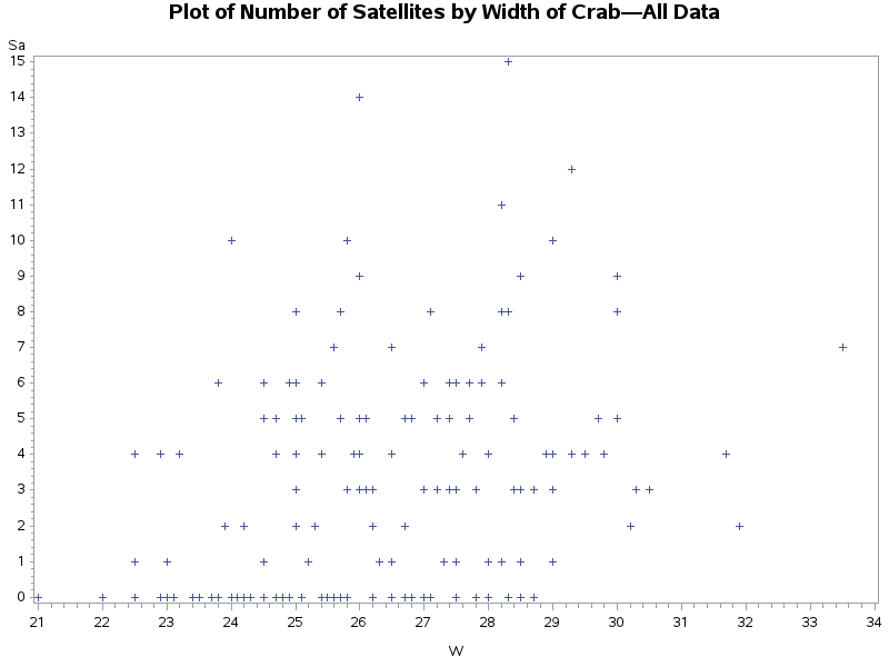
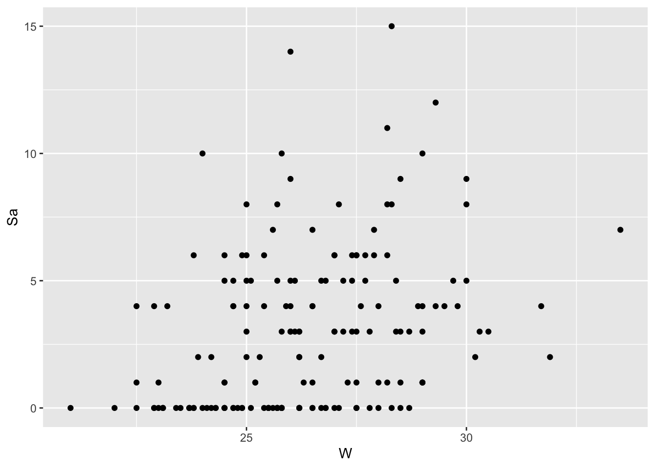
Example 9.1 (Horseshoe Crabs and Satellites)  This problem refers to data from a study of nesting horseshoe crabs (J. Brockmann, Ethology 1996). Each female horseshoe crab in the study had a male crab attached to her in her nest. The study investigated factors that affect whether the female crab had any other males, called satellites, residing near her. Explanatory variables that are thought to affect this included the female crab’s color, spine condition, and carapace width, and weight. The response outcome for each female crab is the number of satellites. There are 173 females in this study.
Let’s first see if the carapace width can explain the number of satellites attached. We will start by fitting a Poisson regression model with carapace width as the only predictor.
proc genmod data=crab;
model Sa=w / dist=poi link=log obstats;
run;
Model Sa=w specifies the response (Sa) and predictor width (W). Also, note that specifications of Poisson distribution are dist=pois and link=log. The obstats option as before will give us a table of observed and predicted values and residuals. We can use any additional options in GENMOD, e.g., TYPE3, etc.
Here is the output that we should get from running just this part:
Model Information
What do we learn from the “Model Information” section? How is this different from when we fitted logistic regression models? This section gives information on the GLM that’s fitted. More specifically, we see that the response is distributed via Poisson, the link function is log, and the dependent variable is Sa. The number of observations in the data set used is 173.
The GENMOD Procedure
| Model Information | |
|---|---|
| Data Set | WORK.CRAB |
| Distribution | Poisson |
| Link Function | Log |
| Dependent Variable | Sa |
| Number of Observations Read | 173 |
|---|---|
| Number of Observations Used | 173 |
Does the model fit well? What does the Value/DF tell us? Given the value of deviance statistic of 567.879 with 171 df, the p-value is zero and the Value/DF is much bigger than 1, so the model does not fit well. The lack of fit may be due to missing data, predictors, or overdispersion. It should also be noted that the deviance and Pearson tests for lack of fit rely on reasonably large expected Poisson counts, which are mostly below five, in this case, so the test results are not entirely reliable. Still, we’d like to see a better-fitting model if possible.
| Criteria For Assessing Goodness Of Fit | |||
|---|---|---|---|
| Criterion | DF | Value | Value/DF |
| Deviance | 171 | 567.8786 | 3.3209 |
| Scaled Deviance | 171 | 567.8786 | 3.3209 |
| Pearson Chi-Square | 171 | 544.1570 | 3.1822 |
| Scaled Pearson X2 | 171 | 544.1570 | 3.1822 |
| Log Likelihood | 68.4463 | ||
| Full Log Likelihood | -461.5881 | ||
| AIC (smaller is better) | 927.1762 | ||
| AICC (smaller is better) | 927.2468 | ||
| BIC (smaller is better) | 933.4828 | ||
Is width a significant predictor? From the “Analysis of Parameter Estimates” table, with Chi-Square stats of 67.51 (1df), the p-value is 0.0001 and this is significant evidence to reject the null hypothesis that \(\beta_W=0\). We can conclude that the carapace width is a significant predictor of the number of satellites.
| Analysis Of Maximum Likelihood Parameter Estimates | |||||||
|---|---|---|---|---|---|---|---|
| Parameter | DF | Estimate | Standard Error |
Wald 95% Confidence Limits | Wald Chi-Square | Pr > ChiSq | |
| Intercept | 1 | -3.3048 | 0.5422 | -4.3675 | -2.2420 | 37.14 | <.0001 |
| W | 1 | 0.1640 | 0.0200 | 0.1249 | 0.2032 | 67.51 | <.0001 |
| Scale | 0 | 1.0000 | 0.0000 | 1.0000 | 1.0000 | ||
The scale parameter was held fixed.
The estimated model is: \(\log (\mu_i) = -3.3048 + 0.164W_i\)
The standard error of the estimated slope is 0.020, which is small, and the slope is statistically significant.
model = glm(Sa ~ W, family=poisson(link=log), data=hcrabs)
summary(model)
model$fitted.values
rstandard(model)
Just as with logistic regression, the glm function specifies the response (Sa) and predictor width (W) separated by the “~” character. Also, note the specification of the Poisson distribution and link function. The fitted (predicted) values are the estimated Poisson counts, and rstandard reports the standardized deviance residuals.
Here is the output that we should get from the summary command:
Does the model fit well? Given the value of deviance statistic of 567.879 with 171 df, the p-value is zero and the Value/DF is much bigger than 1, so the model does not fit well. The lack of fit may be due to missing data, predictors, or overdispersion. It should also be noted that the deviance and Pearson tests for lack of fit rely on reasonably large expected Poisson counts, which are mostly below five, in this case, so the test results are not entirely reliable. Still, we’d like to see a better-fitting model if possible.
Is width a significant predictor? From the “Coefficients” table, with Chi-Square stat of \(8.216^2=67.50\) (1df), the p-value is 0.0001, and this is significant evidence to reject the null hypothesis that \(\beta_W=0\). We can conclude that the carapace width is a significant predictor of the number of satellites.
The estimated model is: \(\log (\mu_i) = -3.3048 + 0.164W_i\)
The standard error of the estimated slope is 0.020, which is small, and the slope is statistically significant.
Interpretation
Since the estimate of \(\beta > 0\), the wider the carapace is, the greater the number of male satellites (on average). Specifically, for each 1-cm increase in carapace width, the expected number of satellites is multiplied by \(\exp(0.1640) = 1.18\).
Looking at the standardized residuals, we may suspect some outliers (e.g., the 15th observation has a standardized deviance residual of almost 5!), but these seem less obvious in the scatterplot, given the overall variability. Also, with a sample size of 173, such extreme values are more likely to occur just by chance. Still, this is something we can address by adding additional predictors or with an adjustment for overdispersion. From the observations statistics, we can also see the predicted values (estimated mean counts) and the values of the linear predictor, which are the log of the expected counts. For example, for the first observation, the predicted value is \(\hat{\mu}_1=3.810\), and the linear predictor is \(\log(3.810)=1.3377\).
From the above output, we see that width is a significant predictor, but the model does not fit well. We can further assess the lack of fit by plotting residuals or influential points, but let us assume for now that we do not have any other covariates and try to adjust for overdispersion to see if we can improve the model fit.
Strategies to Improve the Fit
Adjusting for Overdispersion
In the above model, we detect a potential problem with overdispersion since the scale factor, e.g., Value/DF, is greater than 1.
What does overdispersion mean for Poisson Regression? What does it tell us about the relationship between the mean and the variance of the Poisson distribution for the number of satellites? Recall that one of the reasons for overdispersion is heterogeneity, where subjects within each predictor combination differ greatly (i.e., even crabs with similar width have a different number of satellites). If that’s the case, which assumption of the Poisson model is violated?
As we saw in logistic regression, if we want to test and adjust for overdispersion we can add a scale parameter by changing scale=none to scale=pearson; see the third part of the SAS program crab.sas labeled ’Adjust for overdispersion by scale=pearson. (As stated earlier we can also fit a negative binomial regression instead)
proc genmod data=crab;
model Sa=w / dist=poi link=log scale=pearson;
output out=data2 p=pred;
run;
proc print;
run;
Below is the output when using scale=pearson. How does this compare to the output above from the earlier stage of the code? Do we have a better fit now? Consider the “Scaled Deviance” and “Scaled Pearson chi-square” statistics. The overall model seems to fit better when we account for possible overdispersion.
The GENMOD Procedure
| Model Information | |
|---|---|
| Data Set | WORK.CRAB |
| Distribution | Poisson |
| Link Function | Log |
| Dependent Variable | Sa |
| Number of Observations Read | 173 |
|---|---|
| Number of Observations Used | 173 |
| Criteria For Assessing Goodness Of Fit | |||
|---|---|---|---|
| Criterion | DF | Value | Value/DF |
| Deviance | 171 | 567.8786 | 3.3209 |
| Scaled Deviance | 171 | 567.8786 | 3.3209 |
| Pearson Chi-Square | 171 | 544.1570 | 3.1822 |
| Scaled Pearson X2 | 171 | 544.1570 | 3.1822 |
| Log Likelihood | 68.4463 | ||
| Full Log Likelihood | -461.5881 | ||
| AIC (smaller is better) | 927.1762 | ||
| AICC (smaller is better) | 927.2468 | ||
| BIC (smaller is better) | 933.4828 | ||
| Algorithm converged. |
| Analysis Of Maximum Likelihood Parameter Estimates | |||||||
|---|---|---|---|---|---|---|---|
| Parameter | DF | Estimate | Standard Error |
Wald 95% Confidence Limits | Wald Chi-Square | Pr > ChiSq | |
| Intercept | 1 | -3.3048 | 0.5422 | -4.3675 | -2.2420 | 37.14 | <.0001 |
| W | 1 | 0.1640 | 0.0200 | 0.1249 | 0.2032 | 67.51 | <.0001 |
| Scale | 0 | 1.0000 | 0.0000 | 1.0000 | 1.0000 | ||
The scale parameter was held fixed.
| Observation Statistics | ||||||||||||||||||||
|---|---|---|---|---|---|---|---|---|---|---|---|---|---|---|---|---|---|---|---|---|
| Observation | Sa | W | Predicted Value | Linear Predictor | Standard Error of the Linear Predictor | HessWgt | Lower | Upper | Raw Residual | Pearson Residual | Deviance Residual | Std Deviance Residual | Std Pearson Residual | Likelihood Residual | Leverage | CookD | DFBETA_Intercept | DFBETA_W | DFBETAS_Intercept | DFBETAS_W |
| 1 | 8 | 28.3 | 3.8103412 | 1.3377187 | 0.0508497 | 3.8103412 | 3.4488993 | 4.2096618 | 4.1896588 | 2.1463312 | 1.867685 | 1.8769541 | 2.1569832 | 1.8799166 | 0.0098524 | 0.0231475 | -0.047889 | 0.0020788 | -0.088316 | 0.1041199 |
| 2 | 0 | 22.5 | 1.4714631 | 0.3862572 | 0.1014703 | 1.4714631 | 1.2060844 | 1.7952339 | -1.471463 | -1.213039 | -1.715496 | -1.728641 | -1.222334 | -1.722081 | 0.0151505 | 0.0114923 | -0.07659 | 0.0027203 | -0.141247 | 0.1362502 |
| 3 | 9 | 26 | 2.6127806 | 0.960415 | 0.0493403 | 2.6127806 | 2.371944 | 2.8780708 | 6.3872194 | 3.9514852 | 3.0802813 | 3.0901247 | 3.9641126 | 3.0964636 | 0.0063607 | 0.0502967 | 0.0867684 | -0.002735 | 0.160018 | -0.137005 |
| 4 | 0 | 24.8 | 2.145904 | 0.7635609 | 0.0634803 | 2.145904 | 1.8948542 | 2.4302156 | -2.145904 | -1.46489 | -2.071668 | -2.080684 | -1.471266 | -2.076181 | 0.0086474 | 0.0094409 | -0.057245 | 0.0019565 | -0.105571 | 0.0979966 |
| 5 | 4 | 26 | 2.6127806 | 0.960415 | 0.0493403 | 2.6127806 | 2.371944 | 2.8780708 | 1.3872194 | 0.8582102 | 0.795359 | 0.7979006 | 0.8609527 | 0.7983174 | 0.0063607 | 0.0023725 | 0.0188449 | -0.000594 | 0.0347538 | -0.029756 |
| 6 | 0 | 23.8 | 1.8212368 | 0.5995158 | 0.078969 | 1.8212368 | 1.5600837 | 2.1261061 | -1.821237 | -1.349532 | -1.908527 | -1.919458 | -1.357262 | -1.914 | 0.0113574 | 0.0105813 | -0.068593 | 0.0023994 | -0.126499 | 0.1201774 |
| 7 | 0 | 26.5 | 2.8361218 | 1.0424376 | 0.0459193 | 2.8361218 | 2.5920195 | 3.1032124 | -2.836122 | -1.684079 | -2.381647 | -2.388801 | -1.689137 | -2.385227 | 0.0059802 | 0.0085826 | -0.023121 | 0.0006455 | -0.042639 | 0.0323289 |
| 8 | 0 | 24.7 | 2.1109887 | 0.7471564 | 0.0649192 | 2.1109887 | 1.8587739 | 2.3974262 | -2.110989 | -1.452924 | -2.054745 | -2.063947 | -1.459431 | -2.059351 | 0.0088968 | 0.0095598 | -0.058626 | 0.0020101 | -0.108118 | 0.1006789 |
| 9 | 0 | 23.7 | 1.791604 | 0.5831113 | 0.0806262 | 1.791604 | 1.5297234 | 2.0983173 | -1.791604 | -1.338508 | -1.892936 | -1.904057 | -1.346371 | -1.898505 | 0.0116465 | 0.0106803 | -0.069453 | 0.0024333 | -0.128084 | 0.1218758 |
| 10 | 0 | 25.6 | 2.446839 | 0.894797 | 0.0532791 | 2.446839 | 2.2042158 | 2.7161684 | -2.446839 | -1.564238 | -2.212166 | -2.219889 | -1.569698 | -2.216031 | 0.0069458 | 0.0086169 | -0.043893 | 0.0014414 | -0.080947 | 0.0721929 |
| 11 | 0 | 24.3 | 1.9769166 | 0.6815384 | 0.0709455 | 1.9769166 | 1.7202811 | 2.2718377 | -1.976917 | -1.406029 | -1.988425 | -1.998392 | -1.413077 | -1.993415 | 0.0099504 | 0.0100342 | -0.063579 | 0.0022028 | -0.117251 | 0.1103316 |
| 12 | 0 | 25.8 | 2.5284488 | 0.927606 | 0.051192 | 2.5284488 | 2.28707 | 2.7953029 | -2.528449 | -1.59011 | -2.248755 | -2.256242 | -1.595404 | -2.252502 | 0.0066261 | 0.008489 | -0.03985 | 0.001286 | -0.073491 | 0.0644132 |
| 13 | 11 | 28.2 | 3.7483443 | 1.3213142 | 0.0499141 | 3.7483443 | 3.3990103 | 4.1335812 | 7.2516557 | 3.7455659 | 3.0300943 | 3.0443428 | 3.7631787 | 3.0518391 | 0.0093387 | 0.0667485 | -0.074947 | 0.0033044 | -0.138217 | 0.1655075 |
| 14 | 0 | 21 | 1.1504919 | 0.1401896 | 0.1290549 | 1.1504919 | 0.893371 | 1.4816146 | -1.150492 | -1.07261 | -1.516899 | -1.531645 | -1.083036 | -1.52429 | 0.0191616 | 0.0114575 | -0.079112 | 0.0028369 | -0.145898 | 0.1420936 |
| 15 | 14 | 26 | 2.6127806 | 0.960415 | 0.0493403 | 2.6127806 | 2.371944 | 2.8780708 | 11.387219 | 7.0447602 | 4.9221485 | 4.9378778 | 7.0672725 | 4.9543153 | 0.0063607 | 0.1598642 | 0.1546918 | -0.004877 | 0.2852822 | -0.244255 |
| 16 | 8 | 27.1 | 3.129473 | 1.1408646 | 0.0445041 | 3.129473 | 2.8680665 | 3.4147051 | 4.870527 | 2.7532164 | 2.296993 | 2.304145 | 2.7617889 | 2.3072612 | 0.0061983 | 0.0237861 | 0.0079875 | 0.0000634 | 0.0147306 | 0.0031776 |
| 17 | 1 | 25.2 | 2.2914366 | 0.829179 | 0.0580554 | 2.2914366 | 2.0449892 | 2.5675841 | -1.291437 | -0.853138 | -0.961517 | -0.965252 | -0.856451 | -0.964459 | 0.0077231 | 0.0028545 | -0.028802 | 0.0009689 | -0.053116 | 0.048527 |
| 18 | 1 | 29 | 4.2740006 | 1.4525503 | 0.0588966 | 4.2740006 | 3.8080417 | 4.796975 | -3.274001 | -1.583658 | -1.908638 | -1.922946 | -1.59553 | -1.9185 | 0.0148257 | 0.019155 | 0.0627111 | -0.00256 | 0.1156515 | -0.12822 |
| 19 | 0 | 24.7 | 2.1109887 | 0.7471564 | 0.0649192 | 2.1109887 | 1.8587739 | 2.3974262 | -2.110989 | -1.452924 | -2.054745 | -2.063947 | -1.459431 | -2.059351 | 0.0088968 | 0.0095598 | -0.058626 | 0.0020101 | -0.108118 | 0.1006789 |
| 20 | 5 | 27.4 | 3.2873381 | 1.1900781 | 0.0449918 | 3.2873381 | 3.0098669 | 3.5903886 | 1.7126619 | 0.9446033 | 0.8765123 | 0.8794433 | 0.947762 | 0.8799154 | 0.0066544 | 0.0030087 | -0.002771 | 0.0002285 | -0.00511 | 0.0114448 |
| 21 | 4 | 23.2 | 1.6505173 | 0.5010888 | 0.0891212 | 1.6505173 | 1.3859898 | 1.9655322 | 2.3494827 | 1.8287831 | 1.543593 | 1.5538113 | 1.8408893 | 1.557917 | 0.0131094 | 0.0225081 | 0.1040575 | -0.00367 | 0.1919026 | -0.183829 |
| 22 | 3 | 25 | 2.2174767 | 0.7963699 | 0.0606971 | 2.2174767 | 1.9687636 | 2.4976096 | 0.7825233 | 0.525494 | 0.498405 | 0.5004534 | 0.5276537 | 0.5006816 | 0.0081695 | 0.0011466 | 0.0191623 | -0.00065 | 0.0353391 | -0.032568 |
| 23 | 1 | 22.5 | 1.4714631 | 0.3862572 | 0.1014703 | 1.4714631 | 1.2060844 | 1.7952339 | -0.471463 | -0.388663 | -0.41281 | -0.415973 | -0.391641 | -0.415615 | 0.0151505 | 0.0011798 | -0.02454 | 0.0008716 | -0.045256 | 0.0436552 |
| 24 | 2 | 26.7 | 2.9307155 | 1.0752466 | 0.0451003 | 2.9307155 | 2.6827746 | 3.201571 | -0.930715 | -0.543663 | -0.57709 | -0.578818 | -0.545291 | -0.578624 | 0.0059612 | 0.0008916 | -0.005567 | 0.0001372 | -0.010266 | 0.0068703 |
| 25 | 3 | 25.8 | 2.5284488 | 0.927606 | 0.051192 | 2.5284488 | 2.28707 | 2.7953029 | 0.4715512 | 0.2965526 | 0.287985 | 0.2889439 | 0.29754 | 0.2890017 | 0.0066261 | 0.0002953 | 0.0074319 | -0.00024 | 0.013706 | -0.012013 |
| 26 | 0 | 26.2 | 2.6999251 | 0.993224 | 0.0477514 | 2.6999251 | 2.4587007 | 2.9648162 | -2.699925 | -1.643145 | -2.323758 | -2.330944 | -1.648226 | -2.327354 | 0.0061564 | 0.0084141 | -0.030808 | 0.0009394 | -0.056816 | 0.0470536 |
| 27 | 3 | 28.7 | 4.0687538 | 1.4033368 | 0.0551588 | 4.0687538 | 3.6518264 | 4.5332816 | -1.068754 | -0.529843 | -0.556022 | -0.559496 | -0.533153 | -0.559178 | 0.0123792 | 0.0017815 | 0.0169177 | -0.000704 | 0.0311996 | -0.03527 |
| 28 | 5 | 26.8 | 2.9791889 | 1.0916511 | 0.0448188 | 2.9791889 | 2.7286523 | 3.2527291 | 2.0208111 | 1.1707837 | 1.0659484 | 1.0691523 | 1.1743028 | 1.0698123 | 0.0059844 | 0.004151 | 0.0098938 | -0.000217 | 0.0182461 | -0.010859 |
| 29 | 0 | 27.5 | 3.34171 | 1.2064827 | 0.0453294 | 3.34171 | 3.0576257 | 3.6521886 | -3.34171 | -1.828034 | -2.585231 | -2.594153 | -1.834343 | -2.589696 | 0.0068664 | 0.0116319 | 0.0090379 | -0.00058 | 0.0166677 | -0.029054 |
| 30 | 0 | 24.9 | 2.1813969 | 0.7799654 | 0.0620722 | 2.1813969 | 1.9315179 | 2.4636025 | -2.181397 | -1.476955 | -2.08873 | -2.097564 | -1.483201 | -2.093152 | 0.0084048 | 0.0093232 | -0.055804 | 0.0019007 | -0.102914 | 0.0952009 |
| 31 | 4 | 29.3 | 4.4896009 | 1.5017638 | 0.0629831 | 4.4896009 | 3.9682261 | 5.0794779 | -0.489601 | -0.231067 | -0.23547 | -0.237595 | -0.233153 | -0.237517 | 0.0178097 | 0.0004928 | 0.0110199 | -0.000444 | 0.0203229 | -0.022218 |
| 32 | 0 | 25.8 | 2.5284488 | 0.927606 | 0.051192 | 2.5284488 | 2.28707 | 2.7953029 | -2.528449 | -1.59011 | -2.248755 | -2.256242 | -1.595404 | -2.252502 | 0.0066261 | 0.008489 | -0.03985 | 0.001286 | -0.073491 | 0.0644132 |
| 33 | 0 | 25.7 | 2.4873092 | 0.9112015 | 0.0522078 | 2.4873092 | 2.2453828 | 2.7553018 | -2.487309 | -1.577121 | -2.230385 | -2.237984 | -1.582494 | -2.234188 | 0.0067796 | 0.0085469 | -0.04191 | 0.0013651 | -0.07729 | 0.0683748 |
| 34 | 8 | 25.7 | 2.4873092 | 0.9112015 | 0.0522078 | 2.4873092 | 2.2453828 | 2.7553018 | 5.5126908 | 3.4954149 | 2.7688371 | 2.7782709 | 3.5073242 | 2.7838564 | 0.0067796 | 0.0419834 | 0.0928854 | -0.003026 | 0.1712989 | -0.151541 |
| 35 | 5 | 26.7 | 2.9307155 | 1.0752466 | 0.0451003 | 2.9307155 | 2.6827746 | 3.201571 | 2.0692845 | 1.2087413 | 1.0969705 | 1.1002548 | 1.2123603 | 1.1009569 | 0.0059612 | 0.0044072 | 0.012377 | -0.000305 | 0.0228255 | -0.015275 |
| 36 | 0 | 23.7 | 1.791604 | 0.5831113 | 0.0806262 | 1.791604 | 1.5297234 | 2.0983173 | -1.791604 | -1.338508 | -1.892936 | -1.904057 | -1.346371 | -1.898505 | 0.0116465 | 0.0106803 | -0.069453 | 0.0024333 | -0.128084 | 0.1218758 |
| 37 | 0 | 26.8 | 2.9791889 | 1.0916511 | 0.0448188 | 2.9791889 | 2.7286523 | 3.2527291 | -2.979189 | -1.726033 | -2.440979 | -2.448316 | -1.731221 | -2.44465 | 0.0059844 | 0.009022 | -0.014586 | 0.0003196 | -0.026899 | 0.0160083 |
| 38 | 6 | 27.5 | 3.34171 | 1.2064827 | 0.0453294 | 3.34171 | 3.0576257 | 3.6521886 | 2.65829 | 1.4541794 | 1.3064233 | 1.3109317 | 1.4591977 | 1.3120069 | 0.0068664 | 0.0073607 | -0.00719 | 0.0004614 | -0.013259 | 0.0231117 |
| 39 | 0 | 23.4 | 1.7055673 | 0.5338978 | 0.0856847 | 1.7055673 | 1.441896 | 2.0174548 | -1.705567 | -1.305974 | -1.846926 | -1.858599 | -1.314228 | -1.852772 | 0.012522 | 0.0109511 | -0.071767 | 0.002525 | -0.132352 | 0.1264711 |
| 40 | 6 | 27.9 | 3.5683407 | 1.2721007 | 0.047502 | 3.5683407 | 3.2511162 | 3.916518 | 2.4316593 | 1.2872698 | 1.1715744 | 1.1763197 | 1.2924837 | 1.1773008 | 0.0080518 | 0.0067799 | -0.017164 | 0.0008135 | -0.031654 | 0.0407438 |
| 41 | 3 | 27.5 | 3.34171 | 1.2064827 | 0.0453294 | 3.34171 | 3.0576257 | 3.6521886 | -0.34171 | -0.186928 | -0.190257 | -0.190914 | -0.187573 | -0.190891 | 0.0068664 | 0.0001216 | 0.0009242 | -0.000059 | 0.0017044 | -0.002971 |
| 42 | 5 | 26.1 | 2.6559955 | 0.9768195 | 0.0485113 | 2.6559955 | 2.4150964 | 2.9209236 | 2.3440045 | 1.4382844 | 1.279912 | 1.2839309 | 1.4428006 | 1.2849849 | 0.0062505 | 0.0065466 | 0.0292941 | -0.00091 | 0.054024 | -0.045564 |
| 43 | 6 | 27.7 | 3.4531666 | 1.2392917 | 0.0462564 | 3.4531666 | 3.1538717 | 3.780864 | 2.5468334 | 1.3705402 | 1.2393332 | 1.2439372 | 1.3756316 | 1.2449613 | 0.0073886 | 0.007043 | -0.012428 | 0.0006469 | -0.022921 | 0.0323998 |
| 44 | 5 | 30 | 5.0359157 | 1.6165954 | 0.0735395 | 5.0359157 | 4.3599504 | 5.8166825 | -0.035916 | -0.016005 | -0.016024 | -0.016246 | -0.016227 | -0.016246 | 0.0272345 | 3.6861E-6 | 0.0010951 | -0.000043 | 0.0020195 | -0.002162 |
| 45 | 9 | 28.5 | 3.9374281 | 1.3705277 | 0.0528975 | 3.9374281 | 3.5496552 | 4.3675623 | 5.0625719 | 2.5513197 | 2.1806878 | 2.1928008 | 2.5654915 | 2.1972514 | 0.0110175 | 0.0366612 | -0.068981 | 0.002923 | -0.127214 | 0.1464019 |
| 46 | 4 | 28.9 | 4.2044596 | 1.4361458 | 0.0576085 | 4.2044596 | 3.755552 | 4.7070259 | -0.20446 | -0.099713 | -0.100538 | -0.101247 | -0.100416 | -0.101235 | 0.0139535 | 0.0000713 | 0.0036891 | -0.000151 | 0.0068034 | -0.007586 |
| 47 | 6 | 28.2 | 3.7483443 | 1.3213142 | 0.0499141 | 3.7483443 | 3.3990103 | 4.1335812 | 2.2516557 | 1.1630068 | 1.0686588 | 1.0736839 | 1.1684756 | 1.0746079 | 0.0093387 | 0.0064353 | -0.023271 | 0.001026 | -0.042917 | 0.0513904 |
| 48 | 4 | 25 | 2.2174767 | 0.7963699 | 0.0606971 | 2.2174767 | 1.9687636 | 2.4976096 | 1.7825233 | 1.1970318 | 1.0744063 | 1.078822 | 1.2019515 | 1.0798848 | 0.0081695 | 0.0059498 | 0.0436502 | -0.001481 | 0.0804995 | -0.074187 |
| 49 | 3 | 28.5 | 3.9374281 | 1.3705277 | 0.0528975 | 3.9374281 | 3.5496552 | 4.3675623 | -0.937428 | -0.472424 | -0.493319 | -0.496059 | -0.475048 | -0.495832 | 0.0110175 | 0.001257 | 0.0127731 | -0.000541 | 0.023556 | -0.027109 |
| 50 | 3 | 30.3 | 5.2899506 | 1.6658089 | 0.0783919 | 5.2899506 | 4.5365357 | 6.1684905 | -2.289951 | -0.995635 | -1.084768 | -1.102842 | -1.012224 | -1.100013 | 0.0325083 | 0.0172135 | 0.0778629 | -0.00305 | 0.1435946 | -0.152753 |
| 51 | 5 | 24.7 | 2.1109887 | 0.7471564 | 0.0649192 | 2.1109887 | 1.8587739 | 2.3974262 | 2.8890113 | 1.9884116 | 1.6866512 | 1.6942045 | 1.9973163 | 1.69714 | 0.0088968 | 0.0179051 | 0.0802329 | -0.002751 | 0.1479652 | -0.137785 |
| 52 | 5 | 27.7 | 3.4531666 | 1.2392917 | 0.0462564 | 3.4531666 | 3.1538717 | 3.780864 | 1.5468334 | 0.8324052 | 0.7796125 | 0.7825087 | 0.8354975 | 0.7829133 | 0.0073886 | 0.002598 | -0.007548 | 0.0003929 | -0.013921 | 0.0196782 |
| 53 | 6 | 27.4 | 3.2873381 | 1.1900781 | 0.0449918 | 3.2873381 | 3.0098669 | 3.5903886 | 2.7126619 | 1.4961443 | 1.3397209 | 1.3442008 | 1.5011473 | 1.3453057 | 0.0066544 | 0.0075479 | -0.004389 | 0.0003619 | -0.008093 | 0.0181272 |
| 54 | 4 | 22.9 | 1.5712559 | 0.4518753 | 0.0943581 | 1.5712559 | 1.3059579 | 1.8904478 | 2.4287441 | 1.937574 | 1.6179817 | 1.6294193 | 1.9512708 | 1.634359 | 0.0139896 | 0.0270103 | 0.1156371 | -0.004092 | 0.2132575 | -0.204953 |
| 55 | 5 | 25.7 | 2.4873092 | 0.9112015 | 0.0522078 | 2.4873092 | 2.2453828 | 2.7553018 | 2.5126908 | 1.5932141 | 1.3989219 | 1.4036882 | 1.5986424 | 1.405101 | 0.0067796 | 0.0087222 | 0.0423373 | -0.001379 | 0.0780782 | -0.069073 |
| 56 | 15 | 28.3 | 3.8103412 | 1.3377187 | 0.0508497 | 3.8103412 | 3.4488993 | 4.2096618 | 11.189659 | 5.7323792 | 4.3278894 | 4.3493682 | 5.7608284 | 4.365501 | 0.0098524 | 0.1651128 | -0.1279 | 0.005552 | -0.235874 | 0.2780814 |
| 57 | 3 | 27.2 | 3.1812339 | 1.1572691 | 0.0445779 | 3.1812339 | 2.915082 | 3.4716858 | -0.181234 | -0.101611 | -0.1026 | -0.102925 | -0.101934 | -0.102919 | 0.0063217 | 0.0000331 | -0.0001 | -9.631E-6 | -0.000185 | -0.000482 |
| 58 | 3 | 26.2 | 2.6999251 | 0.993224 | 0.0477514 | 2.6999251 | 2.4587007 | 2.9648162 | 0.3000749 | 0.1826223 | 0.1793871 | 0.1799419 | 0.183187 | 0.179962 | 0.0061564 | 0.0001039 | 0.003424 | -0.000104 | 0.0063146 | -0.00523 |
| 59 | 0 | 27.8 | 3.5102813 | 1.2556962 | 0.0468408 | 3.5102813 | 3.2023658 | 3.8478037 | -3.510281 | -1.873574 | -2.649634 | -2.659897 | -1.880831 | -2.654771 | 0.0077018 | 0.0137284 | 0.0209523 | -0.001033 | 0.0386401 | -0.051733 |
| 60 | 0 | 25.5 | 2.4070273 | 0.8783925 | 0.0544027 | 2.4070273 | 2.1635821 | 2.6778647 | -2.407027 | -1.55146 | -2.194095 | -2.201953 | -1.557016 | -2.198028 | 0.007124 | 0.0086973 | -0.045802 | 0.0015148 | -0.084469 | 0.0758713 |
| 61 | 0 | 27.1 | 3.129473 | 1.1408646 | 0.0445041 | 3.129473 | 2.8680665 | 3.4147051 | -3.129473 | -1.769032 | -2.501789 | -2.509578 | -1.77454 | -2.505686 | 0.0061983 | 0.0098201 | -0.005132 | -0.000041 | -0.009465 | -0.002042 |
| 62 | 5 | 24.5 | 2.0428531 | 0.7143474 | 0.0678818 | 2.0428531 | 1.7883644 | 2.3335561 | 2.9571469 | 2.0689707 | 1.7425875 | 1.7508477 | 2.0787779 | 1.7542204 | 0.0094133 | 0.0205323 | 0.0886098 | -0.003055 | 0.1634139 | -0.153028 |
| 63 | 3 | 27 | 3.0785543 | 1.1244601 | 0.0445198 | 3.0785543 | 2.8213143 | 3.3592488 | -0.078554 | -0.044771 | -0.044963 | -0.045101 | -0.044908 | -0.0451 | 0.0061017 | 6.1906E-6 | -0.000214 | 2.1274E-6 | -0.000395 | 0.0001066 |
| 64 | 5 | 26 | 2.6127806 | 0.960415 | 0.0493403 | 2.6127806 | 2.371944 | 2.8780708 | 2.3872194 | 1.4768652 | 1.3098817 | 1.3140676 | 1.4815847 | 1.3152005 | 0.0063607 | 0.0070259 | 0.0324296 | -0.001022 | 0.0598066 | -0.051206 |
| 65 | 1 | 28 | 3.6273603 | 1.2885052 | 0.0482369 | 3.6273603 | 3.3001325 | 3.9870347 | -2.62736 | -1.379508 | -1.636371 | -1.643321 | -1.385367 | -1.641313 | 0.0084401 | 0.0081683 | 0.0214118 | -0.000985 | 0.0394876 | -0.04933 |
| 66 | 8 | 30 | 5.0359157 | 1.6165954 | 0.0735395 | 5.0359157 | 4.3599504 | 5.8166825 | 2.9640843 | 1.3208434 | 1.2154711 | 1.2323684 | 1.3392056 | 1.2354005 | 0.0272345 | 0.0251059 | -0.090376 | 0.0035618 | -0.16667 | 0.1783995 |
| 67 | 10 | 29 | 4.2740006 | 1.4525503 | 0.0588966 | 4.2740006 | 3.8080417 | 4.796975 | 5.7259994 | 2.7697082 | 2.3555673 | 2.3732253 | 2.7904708 | 2.3799456 | 0.0148257 | 0.0585905 | -0.109677 | 0.0044772 | -0.202267 | 0.2242482 |
| 68 | 0 | 26.2 | 2.6999251 | 0.993224 | 0.0477514 | 2.6999251 | 2.4587007 | 2.9648162 | -2.699925 | -1.643145 | -2.323758 | -2.330944 | -1.648226 | -2.327354 | 0.0061564 | 0.0084141 | -0.030808 | 0.0009394 | -0.056816 | 0.0470536 |
| 69 | 0 | 26.5 | 2.8361218 | 1.0424376 | 0.0459193 | 2.8361218 | 2.5920195 | 3.1032124 | -2.836122 | -1.684079 | -2.381647 | -2.388801 | -1.689137 | -2.385227 | 0.0059802 | 0.0085826 | -0.023121 | 0.0006455 | -0.042639 | 0.0323289 |
| 70 | 3 | 26.2 | 2.6999251 | 0.993224 | 0.0477514 | 2.6999251 | 2.4587007 | 2.9648162 | 0.3000749 | 0.1826223 | 0.1793871 | 0.1799419 | 0.183187 | 0.179962 | 0.0061564 | 0.0001039 | 0.003424 | -0.000104 | 0.0063146 | -0.00523 |
| 71 | 7 | 25.6 | 2.446839 | 0.894797 | 0.0532791 | 2.446839 | 2.2042158 | 2.7161684 | 4.553161 | 2.9107862 | 2.3683881 | 2.3766563 | 2.920948 | 2.380866 | 0.0069458 | 0.0298376 | 0.0816777 | -0.002682 | 0.1506298 | -0.134339 |
| 72 | 1 | 23 | 1.5972442 | 0.4682798 | 0.0926023 | 1.5972442 | 1.3321345 | 1.9151136 | -0.597244 | -0.47257 | -0.507867 | -0.511381 | -0.47584 | -0.510911 | 0.0136967 | 0.0015722 | -0.027774 | 0.0009818 | -0.051221 | 0.0491755 |
| 73 | 0 | 23 | 1.5972442 | 0.4682798 | 0.0926023 | 1.5972442 | 1.3321345 | 1.9151136 | -1.597244 | -1.263821 | -1.787313 | -1.79968 | -1.272566 | -1.793507 | 0.0136967 | 0.0112444 | -0.074278 | 0.0026257 | -0.136983 | 0.1315128 |
| 74 | 6 | 25.4 | 2.3678633 | 0.861988 | 0.0555752 | 2.3678633 | 2.1234935 | 2.640355 | 3.6321367 | 2.3603906 | 1.9730647 | 1.9803195 | 2.3690695 | 1.9834391 | 0.0073134 | 0.0206744 | 0.0730755 | -0.002432 | 0.1347655 | -0.121815 |
| 75 | 0 | 24.2 | 1.9447508 | 0.6651339 | 0.0725113 | 1.9447508 | 1.6871055 | 2.2417424 | -1.944751 | -1.394543 | -1.972182 | -1.982343 | -1.401728 | -1.977269 | 0.0102253 | 0.0101493 | -0.064681 | 0.0022459 | -0.119285 | 0.1124894 |
| 76 | 0 | 22.9 | 1.5712559 | 0.4518753 | 0.0943581 | 1.5712559 | 1.3059579 | 1.8904478 | -1.571256 | -1.253497 | -1.772713 | -1.785245 | -1.262359 | -1.77899 | 0.0139896 | 0.0113047 | -0.07481 | 0.0026473 | -0.137965 | 0.132593 |
| 77 | 3 | 26 | 2.6127806 | 0.960415 | 0.0493403 | 2.6127806 | 2.371944 | 2.8780708 | 0.3872194 | 0.2395552 | 0.2339761 | 0.2347238 | 0.2403207 | 0.2347598 | 0.0063607 | 0.0001849 | 0.0052603 | -0.000166 | 0.0097009 | -0.008306 |
| 78 | 4 | 25.4 | 2.3678633 | 0.861988 | 0.0555752 | 2.3678633 | 2.1234935 | 2.640355 | 1.6321367 | 1.060665 | 0.9644572 | 0.9680034 | 1.0645649 | 0.9687445 | 0.0073134 | 0.0041747 | 0.0328372 | -0.001093 | 0.0605582 | -0.054739 |
| 79 | 0 | 25.7 | 2.4873092 | 0.9112015 | 0.0522078 | 2.4873092 | 2.2453828 | 2.7553018 | -2.487309 | -1.577121 | -2.230385 | -2.237984 | -1.582494 | -2.234188 | 0.0067796 | 0.0085469 | -0.04191 | 0.0013651 | -0.07729 | 0.0683748 |
| 80 | 5 | 25.1 | 2.2541534 | 0.8127744 | 0.0593574 | 2.2541534 | 2.0065887 | 2.5322615 | 2.7458466 | 1.8288772 | 1.5731946 | 1.5794793 | 1.8361833 | 1.5816822 | 0.0079421 | 0.0134958 | 0.0642381 | -0.002171 | 0.1184677 | -0.108727 |
| 81 | 0 | 24.5 | 2.0428531 | 0.7143474 | 0.0678818 | 2.0428531 | 1.7883644 | 2.3335561 | -2.042853 | -1.429284 | -2.021313 | -2.030894 | -1.436059 | -2.026109 | 0.0094133 | 0.0097987 | -0.061213 | 0.0021106 | -0.112889 | 0.1057149 |
| 82 | 0 | 27.5 | 3.34171 | 1.2064827 | 0.0453294 | 3.34171 | 3.0576257 | 3.6521886 | -3.34171 | -1.828034 | -2.585231 | -2.594153 | -1.834343 | -2.589696 | 0.0068664 | 0.0116319 | 0.0090379 | -0.00058 | 0.0166677 | -0.029054 |
| 83 | 0 | 23.1 | 1.6236623 | 0.4846843 | 0.0908565 | 1.6236623 | 1.3588094 | 1.9401391 | -1.623662 | -1.27423 | -1.802033 | -1.814233 | -1.282856 | -1.808143 | 0.0134032 | 0.0111788 | -0.073708 | 0.0026027 | -0.135933 | 0.1303624 |
| 84 | 4 | 25.9 | 2.5702689 | 0.9440105 | 0.050235 | 2.5702689 | 2.3292626 | 2.8362119 | 1.4297311 | 0.8917951 | 0.8238984 | 0.8265834 | 0.8947014 | 0.8270433 | 0.0064862 | 0.002613 | 0.0209776 | -0.00067 | 0.0386868 | -0.033545 |
| 85 | 0 | 25.8 | 2.5284488 | 0.927606 | 0.051192 | 2.5284488 | 2.28707 | 2.7953029 | -2.528449 | -1.59011 | -2.248755 | -2.256242 | -1.595404 | -2.252502 | 0.0066261 | 0.008489 | -0.03985 | 0.001286 | -0.073491 | 0.0644132 |
| 86 | 3 | 27 | 3.0785543 | 1.1244601 | 0.0445198 | 3.0785543 | 2.8213143 | 3.3592488 | -0.078554 | -0.044771 | -0.044963 | -0.045101 | -0.044908 | -0.0451 | 0.0061017 | 6.1906E-6 | -0.000214 | 2.1274E-6 | -0.000395 | 0.0001066 |
| 87 | 0 | 28.5 | 3.9374281 | 1.3705277 | 0.0528975 | 3.9374281 | 3.5496552 | 4.3675623 | -3.937428 | -1.984295 | -2.806217 | -2.821805 | -1.995318 | -2.814022 | 0.0110175 | 0.0221763 | 0.05365 | -0.002273 | 0.0989412 | -0.113864 |
| 88 | 0 | 25.5 | 2.4070273 | 0.8783925 | 0.0544027 | 2.4070273 | 2.1635821 | 2.6778647 | -2.407027 | -1.55146 | -2.194095 | -2.201953 | -1.557016 | -2.198028 | 0.007124 | 0.0086973 | -0.045802 | 0.0015148 | -0.084469 | 0.0758713 |
| 89 | 0 | 23.5 | 1.7337771 | 0.5503023 | 0.0839849 | 1.7337771 | 1.4706359 | 2.0440021 | -1.733777 | -1.31673 | -1.862137 | -1.873629 | -1.324856 | -1.867892 | 0.0122291 | 0.0108654 | -0.071038 | 0.0024961 | -0.131009 | 0.1250204 |
| 90 | 0 | 24 | 1.8819808 | 0.6323249 | 0.0757037 | 1.8819808 | 1.6224678 | 2.1830028 | -1.881981 | -1.371853 | -1.940093 | -1.950641 | -1.379312 | -1.945374 | 0.0107857 | 0.0103718 | -0.066735 | 0.0023263 | -0.123072 | 0.1165171 |
| 91 | 5 | 29.7 | 4.7940801 | 1.5673818 | 0.0688663 | 4.7940801 | 4.1887666 | 5.4868667 | 0.2059199 | 0.0940471 | 0.0933857 | 0.0944657 | 0.0951349 | 0.094481 | 0.0227363 | 0.0001053 | -0.005568 | 0.0002211 | -0.010268 | 0.0110746 |
| 92 | 0 | 26.8 | 2.9791889 | 1.0916511 | 0.0448188 | 2.9791889 | 2.7286523 | 3.2527291 | -2.979189 | -1.726033 | -2.440979 | -2.448316 | -1.731221 | -2.44465 | 0.0059844 | 0.009022 | -0.014586 | 0.0003196 | -0.026899 | 0.0160083 |
| 93 | 0 | 26.7 | 2.9307155 | 1.0752466 | 0.0451003 | 2.9307155 | 2.6827746 | 3.201571 | -2.930715 | -1.711933 | -2.421039 | -2.428288 | -1.717059 | -2.424666 | 0.0059612 | 0.0088404 | -0.017529 | 0.0004319 | -0.032328 | 0.0216338 |
| 94 | 0 | 28.7 | 4.0687538 | 1.4033368 | 0.0551588 | 4.0687538 | 3.6518264 | 4.5332816 | -4.068754 | -2.017115 | -2.852632 | -2.870454 | -2.029717 | -2.861557 | 0.0123792 | 0.0258192 | 0.0644059 | -0.002681 | 0.1187771 | -0.134275 |
| 95 | 0 | 23.1 | 1.6236623 | 0.4846843 | 0.0908565 | 1.6236623 | 1.3588094 | 1.9401391 | -1.623662 | -1.27423 | -1.802033 | -1.814233 | -1.282856 | -1.808143 | 0.0134032 | 0.0111788 | -0.073708 | 0.0026027 | -0.135933 | 0.1303624 |
| 96 | 1 | 29 | 4.2740006 | 1.4525503 | 0.0588966 | 4.2740006 | 3.8080417 | 4.796975 | -3.274001 | -1.583658 | -1.908638 | -1.922946 | -1.59553 | -1.9185 | 0.0148257 | 0.019155 | 0.0627111 | -0.00256 | 0.1156515 | -0.12822 |
| 97 | 0 | 25.5 | 2.4070273 | 0.8783925 | 0.0544027 | 2.4070273 | 2.1635821 | 2.6778647 | -2.407027 | -1.55146 | -2.194095 | -2.201953 | -1.557016 | -2.198028 | 0.007124 | 0.0086973 | -0.045802 | 0.0015148 | -0.084469 | 0.0758713 |
| 98 | 1 | 26.5 | 2.8361218 | 1.0424376 | 0.0459193 | 2.8361218 | 2.5920195 | 3.1032124 | -1.836122 | -1.090283 | -1.259908 | -1.263692 | -1.093557 | -1.262743 | 0.0059802 | 0.0035973 | -0.014969 | 0.0004179 | -0.027605 | 0.0209299 |
| 99 | 1 | 24.5 | 2.0428531 | 0.7143474 | 0.0678818 | 2.0428531 | 1.7883644 | 2.3335561 | -1.042853 | -0.729633 | -0.810562 | -0.814405 | -0.733092 | -0.813677 | 0.0094133 | 0.0025535 | -0.031249 | 0.0010775 | -0.057629 | 0.0539662 |
| 100 | 1 | 28.5 | 3.9374281 | 1.3705277 | 0.0528975 | 3.9374281 | 3.5496552 | 4.3675623 | -2.937428 | -1.480338 | -1.770254 | -1.780088 | -1.488561 | -1.777136 | 0.0110175 | 0.0123424 | 0.0400244 | -0.001696 | 0.0738128 | -0.084946 |
| 101 | 1 | 28.2 | 3.7483443 | 1.3213142 | 0.0499141 | 3.7483443 | 3.3990103 | 4.1335812 | -2.748344 | -1.419552 | -1.689396 | -1.69734 | -1.426227 | -1.695009 | 0.0093387 | 0.0095876 | 0.0284047 | -0.001252 | 0.0523838 | -0.062727 |
| 102 | 1 | 24.5 | 2.0428531 | 0.7143474 | 0.0678818 | 2.0428531 | 1.7883644 | 2.3335561 | -1.042853 | -0.729633 | -0.810562 | -0.814405 | -0.733092 | -0.813677 | 0.0094133 | 0.0025535 | -0.031249 | 0.0010775 | -0.057629 | 0.0539662 |
| 103 | 1 | 27.5 | 3.34171 | 1.2064827 | 0.0453294 | 3.34171 | 3.0576257 | 3.6521886 | -2.34171 | -1.280999 | -1.506803 | -1.512003 | -1.28542 | -1.510563 | 0.0068664 | 0.0057119 | 0.0063333 | -0.000406 | 0.0116799 | -0.020359 |
| 104 | 4 | 24.7 | 2.1109887 | 0.7471564 | 0.0649192 | 2.1109887 | 1.8587739 | 2.3974262 | 1.8890113 | 1.3001444 | 1.155457 | 1.1606315 | 1.3059669 | 1.1620047 | 0.0088968 | 0.007655 | 0.0524611 | -0.001799 | 0.0967486 | -0.090092 |
| 105 | 1 | 25.2 | 2.2914366 | 0.829179 | 0.0580554 | 2.2914366 | 2.0449892 | 2.5675841 | -1.291437 | -0.853138 | -0.961517 | -0.965252 | -0.856451 | -0.964459 | 0.0077231 | 0.0028545 | -0.028802 | 0.0009689 | -0.053116 | 0.048527 |
| 106 | 1 | 27.3 | 3.2338508 | 1.1736736 | 0.0447408 | 3.2338508 | 2.9623511 | 3.5302336 | -2.233851 | -1.242208 | -1.456144 | -1.46088 | -1.246248 | -1.459592 | 0.0064733 | 0.0050597 | 0.0011874 | -0.000208 | 0.0021898 | -0.010436 |
| 107 | 1 | 26.3 | 2.7445814 | 1.0096286 | 0.047064 | 2.7445814 | 2.5027367 | 3.009796 | -1.744581 | -1.05306 | -1.212397 | -1.216099 | -1.056276 | -1.215191 | 0.0060793 | 0.0034121 | -0.018011 | 0.000537 | -0.033217 | 0.0268973 |
| 108 | 1 | 29 | 4.2740006 | 1.4525503 | 0.0588966 | 4.2740006 | 3.8080417 | 4.796975 | -3.274001 | -1.583658 | -1.908638 | -1.922946 | -1.59553 | -1.9185 | 0.0148257 | 0.019155 | 0.0627111 | -0.00256 | 0.1156515 | -0.12822 |
| 109 | 2 | 25.3 | 2.3293365 | 0.8455835 | 0.0567937 | 2.3293365 | 2.0839597 | 2.6036053 | -0.329337 | -0.215786 | -0.221196 | -0.222032 | -0.216601 | -0.221992 | 0.0075133 | 0.0001776 | -0.006985 | 0.0002338 | -0.012882 | 0.01171 |
| 110 | 4 | 26.5 | 2.8361218 | 1.0424376 | 0.0459193 | 2.8361218 | 2.5920195 | 3.1032124 | 1.1638782 | 0.6911067 | 0.6504598 | 0.6524136 | 0.6931825 | 0.6526649 | 0.0059802 | 0.0014454 | 0.0094883 | -0.000265 | 0.0174982 | -0.013267 |
| 111 | 3 | 27.8 | 3.5102813 | 1.2556962 | 0.0468408 | 3.5102813 | 3.2023658 | 3.8478037 | -0.510281 | -0.272357 | -0.279391 | -0.280473 | -0.273412 | -0.280419 | 0.0077018 | 0.0002901 | 0.0030458 | -0.00015 | 0.005617 | -0.00752 |
| 112 | 6 | 27 | 3.0785543 | 1.1244601 | 0.0445198 | 3.0785543 | 2.8213143 | 3.3592488 | 2.9214457 | 1.665039 | 1.4712923 | 1.4758016 | 1.6701422 | 1.477065 | 0.0061017 | 0.0085623 | 0.0079621 | -0.000079 | 0.0146836 | -0.003963 |
| 113 | 0 | 25.7 | 2.4873092 | 0.9112015 | 0.0522078 | 2.4873092 | 2.2453828 | 2.7553018 | -2.487309 | -1.577121 | -2.230385 | -2.237984 | -1.582494 | -2.234188 | 0.0067796 | 0.0085469 | -0.04191 | 0.0013651 | -0.07729 | 0.0683748 |
| 114 | 2 | 25 | 2.2174767 | 0.7963699 | 0.0606971 | 2.2174767 | 1.9687636 | 2.4976096 | -0.217477 | -0.146044 | -0.148534 | -0.149145 | -0.146644 | -0.149124 | 0.0081695 | 0.0000886 | -0.005326 | 0.0001807 | -0.009821 | 0.0090511 |
| 115 | 2 | 31.9 | 6.8776776 | 1.928281 | 0.1062496 | 6.8776776 | 5.5847273 | 8.4699659 | -4.877678 | -1.859911 | -2.19427 | -2.284758 | -1.936611 | -2.259649 | 0.077642 | 0.1578527 | 0.2652591 | -0.010187 | 0.4891899 | -0.510223 |
| 116 | 0 | 23.7 | 1.791604 | 0.5831113 | 0.0806262 | 1.791604 | 1.5297234 | 2.0983173 | -1.791604 | -1.338508 | -1.892936 | -1.904057 | -1.346371 | -1.898505 | 0.0116465 | 0.0106803 | -0.069453 | 0.0024333 | -0.128084 | 0.1218758 |
| 117 | 12 | 29.3 | 4.4896009 | 1.5017638 | 0.0629831 | 4.4896009 | 3.9682261 | 5.0794779 | 7.5103991 | 3.544534 | 2.9282469 | 2.954676 | 3.5765255 | 2.9668911 | 0.0178097 | 0.115972 | -0.169044 | 0.0068047 | -0.311751 | 0.3408246 |
| 118 | 0 | 22 | 1.3555871 | 0.3042347 | 0.1105285 | 1.3555871 | 1.0915544 | 1.683486 | -1.355587 | -1.164297 | -1.646564 | -1.66037 | -1.174059 | -1.653482 | 0.0165606 | 0.0116059 | -0.078096 | 0.0027844 | -0.144024 | 0.1394609 |
| 119 | 5 | 25 | 2.2174767 | 0.7963699 | 0.0606971 | 2.2174767 | 1.9687636 | 2.4976096 | 2.7825233 | 1.8685696 | 1.6017594 | 1.6083425 | 1.8762493 | 1.6107118 | 0.0081695 | 0.014498 | 0.068138 | -0.002312 | 0.1256599 | -0.115805 |
| 120 | 6 | 27 | 3.0785543 | 1.1244601 | 0.0445198 | 3.0785543 | 2.8213143 | 3.3592488 | 2.9214457 | 1.665039 | 1.4712923 | 1.4758016 | 1.6701422 | 1.477065 | 0.0061017 | 0.0085623 | 0.0079621 | -0.000079 | 0.0146836 | -0.003963 |
| 121 | 6 | 23.8 | 1.8212368 | 0.5995158 | 0.078969 | 1.8212368 | 1.5600837 | 2.1261061 | 4.1787632 | 3.0964534 | 2.4391386 | 2.4531089 | 3.1141885 | 2.461614 | 0.0113574 | 0.0557057 | 0.1573847 | -0.005505 | 0.2902483 | -0.275743 |
| 122 | 2 | 30.2 | 5.2038794 | 1.6494044 | 0.0767566 | 5.2038794 | 4.4770498 | 6.0487067 | -3.203879 | -1.40447 | -1.607087 | -1.632305 | -1.426508 | -1.626382 | 0.030659 | 0.032181 | 0.1051644 | -0.004127 | 0.1939438 | -0.206711 |
| 123 | 0 | 26.2 | 2.6999251 | 0.993224 | 0.0477514 | 2.6999251 | 2.4587007 | 2.9648162 | -2.699925 | -1.643145 | -2.323758 | -2.330944 | -1.648226 | -2.327354 | 0.0061564 | 0.0084141 | -0.030808 | 0.0009394 | -0.056816 | 0.0470536 |
| 124 | 2 | 24.2 | 1.9447508 | 0.6651339 | 0.0725113 | 1.9447508 | 1.6871055 | 2.2417424 | 0.0552492 | 0.0396181 | 0.0394327 | 0.0396359 | 0.0398222 | 0.0396378 | 0.0102253 | 8.1914E-6 | 0.0018376 | -0.000064 | 0.0033888 | -0.003196 |
| 125 | 3 | 27.4 | 3.2873381 | 1.1900781 | 0.0449918 | 3.2873381 | 3.0098669 | 3.5903886 | -0.287338 | -0.158479 | -0.160876 | -0.161414 | -0.159009 | -0.161398 | 0.0066544 | 0.0000847 | 0.0004649 | -0.000038 | 0.0008573 | -0.00192 |
| 126 | 0 | 25.4 | 2.3678633 | 0.861988 | 0.0555752 | 2.3678633 | 2.1234935 | 2.640355 | -2.367863 | -1.538786 | -2.176172 | -2.184174 | -1.544444 | -2.180177 | 0.0073134 | 0.0087866 | -0.047639 | 0.0015855 | -0.087856 | 0.0794134 |
| 127 | 3 | 28.4 | 3.8733634 | 1.3541232 | 0.0518453 | 3.8733634 | 3.4991088 | 4.2876473 | -0.873363 | -0.443763 | -0.462235 | -0.46466 | -0.446091 | -0.464471 | 0.0104114 | 0.0010468 | 0.0109406 | -0.000469 | 0.0201767 | -0.023479 |
| 128 | 4 | 22.5 | 1.4714631 | 0.3862572 | 0.1014703 | 1.4714631 | 1.2060844 | 1.7952339 | 2.5285369 | 2.084465 | 1.7155825 | 1.728728 | 2.100437 | 1.7349539 | 0.0151505 | 0.0339349 | 0.1316109 | -0.004674 | 0.2427163 | -0.23413 |
| 129 | 2 | 26.2 | 2.6999251 | 0.993224 | 0.0477514 | 2.6999251 | 2.4587007 | 2.9648162 | -0.699925 | -0.425967 | -0.446702 | -0.448084 | -0.427284 | -0.447958 | 0.0061564 | 0.0005655 | -0.007987 | 0.0002435 | -0.014729 | 0.0121981 |
| 130 | 6 | 24.9 | 2.1813969 | 0.7799654 | 0.0620722 | 2.1813969 | 1.9315179 | 2.4636025 | 3.8186031 | 2.5854562 | 2.1223388 | 2.1313144 | 2.5963903 | 2.1356454 | 0.0084048 | 0.0285696 | 0.0976866 | -0.003327 | 0.1801533 | -0.166652 |
| 131 | 6 | 24.5 | 2.0428531 | 0.7143474 | 0.0678818 | 2.0428531 | 1.7883644 | 2.3335561 | 3.9571469 | 2.7686216 | 2.2393416 | 2.2499565 | 2.7817454 | 2.2555471 | 0.0094133 | 0.0367668 | 0.1185745 | -0.004088 | 0.2186746 | -0.204777 |
| 132 | 0 | 25.1 | 2.2541534 | 0.8127744 | 0.0593574 | 2.2541534 | 2.0065887 | 2.5322615 | -2.254153 | -1.501384 | -2.123277 | -2.13176 | -1.507382 | -2.127523 | 0.0079421 | 0.0090952 | -0.052735 | 0.0017821 | -0.097254 | 0.0892572 |
| 133 | 4 | 28 | 3.6273603 | 1.2885052 | 0.0482369 | 3.6273603 | 3.3001325 | 3.9870347 | 0.3726397 | 0.1956563 | 0.192442 | 0.1932593 | 0.1964872 | 0.1932868 | 0.0084401 | 0.0001643 | -0.003037 | 0.0001397 | -0.005601 | 0.0069966 |
| 134 | 10 | 25.8 | 2.5284488 | 0.927606 | 0.051192 | 2.5284488 | 2.28707 | 2.7953029 | 7.4715512 | 4.6987646 | 3.5435123 | 3.5553108 | 4.7144097 | 3.5642319 | 0.0066261 | 0.0741259 | 0.1177563 | -0.0038 | 0.2171657 | -0.190341 |
| 135 | 7 | 27.9 | 3.5683407 | 1.2721007 | 0.047502 | 3.5683407 | 3.2511162 | 3.916518 | 3.4316593 | 1.8166489 | 1.6031262 | 1.6096195 | 1.824007 | 1.6114596 | 0.0080518 | 0.0135028 | -0.024223 | 0.001148 | -0.044672 | 0.0574994 |
| 136 | 0 | 24.9 | 2.1813969 | 0.7799654 | 0.0620722 | 2.1813969 | 1.9315179 | 2.4636025 | -2.181397 | -1.476955 | -2.08873 | -2.097564 | -1.483201 | -2.093152 | 0.0084048 | 0.0093232 | -0.055804 | 0.0019007 | -0.102914 | 0.0952009 |
| 137 | 5 | 28.4 | 3.8733634 | 1.3541232 | 0.0518453 | 3.8733634 | 3.4991088 | 4.2876473 | 1.1266366 | 0.5724528 | 0.5476072 | 0.5504803 | 0.5754563 | 0.5507462 | 0.0104114 | 0.001742 | -0.014113 | 0.0006047 | -0.026028 | 0.0302876 |
| 138 | 5 | 27.2 | 3.1812339 | 1.1572691 | 0.0445779 | 3.1812339 | 2.915082 | 3.4716858 | 1.8187661 | 1.0197156 | 0.9402955 | 0.9432818 | 1.0229541 | 0.9438066 | 0.0063217 | 0.0033287 | 0.0010082 | 0.0000967 | 0.0018594 | 0.0048411 |
| 139 | 6 | 25 | 2.2174767 | 0.7963699 | 0.0606971 | 2.2174767 | 1.9687636 | 2.4976096 | 3.7825233 | 2.5401074 | 2.092756 | 2.1013571 | 2.5505471 | 2.1054151 | 0.0081695 | 0.0267914 | 0.0926259 | -0.003143 | 0.1708204 | -0.157424 |
| 140 | 6 | 27.5 | 3.34171 | 1.2064827 | 0.0453294 | 3.34171 | 3.0576257 | 3.6521886 | 2.65829 | 1.4541794 | 1.3064233 | 1.3109317 | 1.4591977 | 1.3120069 | 0.0068664 | 0.0073607 | -0.00719 | 0.0004614 | -0.013259 | 0.0231117 |
| 141 | 7 | 33.5 | 8.9419455 | 2.1907532 | 0.1359176 | 8.9419455 | 6.8507601 | 11.671462 | -1.941945 | -0.649413 | -0.675343 | -0.739147 | -0.710767 | -0.734534 | 0.1651898 | 0.0499827 | 0.1568405 | -0.005965 | 0.2892448 | -0.298748 |
| 142 | 3 | 30.5 | 5.4663872 | 1.6986179 | 0.0817107 | 5.4663872 | 4.6574492 | 6.4158271 | -2.466387 | -1.054899 | -1.154444 | -1.176106 | -1.074693 | -1.172559 | 0.0364971 | 0.0218748 | 0.0897332 | -0.003502 | 0.1654856 | -0.175425 |
| 143 | 3 | 29 | 4.2740006 | 1.4525503 | 0.0588966 | 4.2740006 | 3.8080417 | 4.796975 | -1.274001 | -0.616243 | -0.651439 | -0.656323 | -0.620863 | -0.655811 | 0.0148257 | 0.0029004 | 0.0244025 | -0.000996 | 0.0450031 | -0.049894 |
| 144 | 0 | 24.3 | 1.9769166 | 0.6815384 | 0.0709455 | 1.9769166 | 1.7202811 | 2.2718377 | -1.976917 | -1.406029 | -1.988425 | -1.998392 | -1.413077 | -1.993415 | 0.0099504 | 0.0100342 | -0.063579 | 0.0022028 | -0.117251 | 0.1103316 |
| 145 | 0 | 25.8 | 2.5284488 | 0.927606 | 0.051192 | 2.5284488 | 2.28707 | 2.7953029 | -2.528449 | -1.59011 | -2.248755 | -2.256242 | -1.595404 | -2.252502 | 0.0066261 | 0.008489 | -0.03985 | 0.001286 | -0.073491 | 0.0644132 |
| 146 | 8 | 25 | 2.2174767 | 0.7963699 | 0.0606971 | 2.2174767 | 1.9687636 | 2.4976096 | 5.7825233 | 3.883183 | 2.9940105 | 3.0063158 | 3.8991426 | 3.0146812 | 0.0081695 | 0.0626132 | 0.1416016 | -0.004805 | 0.2611412 | -0.240662 |
| 147 | 4 | 31.7 | 6.6556893 | 1.895472 | 0.1026373 | 6.6556893 | 5.442871 | 8.1387563 | -2.655689 | -1.029392 | -1.112635 | -1.15382 | -1.067495 | -1.147979 | 0.0701138 | 0.0429611 | 0.1370903 | -0.005274 | 0.2528215 | -0.264142 |
| 148 | 4 | 29.5 | 4.6393433 | 1.5345728 | 0.0658694 | 4.6393433 | 4.0774475 | 5.2786717 | -0.639343 | -0.296829 | -0.304071 | -0.307178 | -0.299862 | -0.307032 | 0.0201291 | 0.0009236 | 0.0158324 | -0.000633 | 0.029198 | -0.031688 |
| 149 | 10 | 24 | 1.8819808 | 0.6323249 | 0.0757037 | 1.8819808 | 1.6224678 | 2.1830028 | 8.1180192 | 5.9175573 | 4.1435693 | 4.1660974 | 5.9497304 | 4.1893882 | 0.0107857 | 0.192985 | 0.2878633 | -0.010035 | 0.5308764 | -0.502603 |
| 150 | 9 | 30 | 5.0359157 | 1.6165954 | 0.0735395 | 5.0359157 | 4.3599504 | 5.8166825 | 3.9640843 | 1.7664594 | 1.5884448 | 1.6105272 | 1.7910165 | 1.6157098 | 0.0272345 | 0.0449035 | -0.120866 | 0.0047635 | -0.2229 | 0.2385865 |
| 151 | 4 | 27.6 | 3.3969812 | 1.2228872 | 0.0457517 | 3.3969812 | 3.1056266 | 3.7156693 | 0.6030188 | 0.3271781 | 0.318151 | 0.3192882 | 0.3283476 | 0.3193535 | 0.0071106 | 0.0003861 | -0.002287 | 0.0001289 | -0.004217 | 0.0064566 |
| 152 | 0 | 26.2 | 2.6999251 | 0.993224 | 0.0477514 | 2.6999251 | 2.4587007 | 2.9648162 | -2.699925 | -1.643145 | -2.323758 | -2.330944 | -1.648226 | -2.327354 | 0.0061564 | 0.0084141 | -0.030808 | 0.0009394 | -0.056816 | 0.0470536 |
| 153 | 0 | 23.1 | 1.6236623 | 0.4846843 | 0.0908565 | 1.6236623 | 1.3588094 | 1.9401391 | -1.623662 | -1.27423 | -1.802033 | -1.814233 | -1.282856 | -1.808143 | 0.0134032 | 0.0111788 | -0.073708 | 0.0026027 | -0.135933 | 0.1303624 |
| 154 | 0 | 22.9 | 1.5712559 | 0.4518753 | 0.0943581 | 1.5712559 | 1.3059579 | 1.8904478 | -1.571256 | -1.253497 | -1.772713 | -1.785245 | -1.262359 | -1.77899 | 0.0139896 | 0.0113047 | -0.07481 | 0.0026473 | -0.137965 | 0.132593 |
| 155 | 0 | 24.5 | 2.0428531 | 0.7143474 | 0.0678818 | 2.0428531 | 1.7883644 | 2.3335561 | -2.042853 | -1.429284 | -2.021313 | -2.030894 | -1.436059 | -2.026109 | 0.0094133 | 0.0097987 | -0.061213 | 0.0021106 | -0.112889 | 0.1057149 |
| 156 | 4 | 24.7 | 2.1109887 | 0.7471564 | 0.0649192 | 2.1109887 | 1.8587739 | 2.3974262 | 1.8890113 | 1.3001444 | 1.155457 | 1.1606315 | 1.3059669 | 1.1620047 | 0.0088968 | 0.007655 | 0.0524611 | -0.001799 | 0.0967486 | -0.090092 |
| 157 | 0 | 28.3 | 3.8103412 | 1.3377187 | 0.0508497 | 3.8103412 | 3.4488993 | 4.2096618 | -3.810341 | -1.95201 | -2.760558 | -2.774259 | -1.961697 | -2.767417 | 0.0098524 | 0.0191459 | 0.0435531 | -0.001891 | 0.0803205 | -0.094693 |
| 158 | 2 | 23.9 | 1.8513597 | 0.6159203 | 0.0773278 | 1.8513597 | 1.5909967 | 2.1543306 | 0.1486403 | 0.1092424 | 0.1078274 | 0.1084293 | 0.1098521 | 0.1084451 | 0.0110704 | 0.0000675 | 0.0054344 | -0.00019 | 0.0100222 | -0.009505 |
| 159 | 0 | 23.8 | 1.8212368 | 0.5995158 | 0.078969 | 1.8212368 | 1.5600837 | 2.1261061 | -1.821237 | -1.349532 | -1.908527 | -1.919458 | -1.357262 | -1.914 | 0.0113574 | 0.0105813 | -0.068593 | 0.0023994 | -0.126499 | 0.1201774 |
| 160 | 4 | 29.8 | 4.8733733 | 1.5837864 | 0.0704019 | 4.8733733 | 4.245252 | 5.5944304 | -0.873373 | -0.395626 | -0.408424 | -0.413448 | -0.400493 | -0.41314 | 0.0241545 | 0.0019851 | 0.024614 | -0.000975 | 0.045393 | -0.048826 |
| 161 | 4 | 26.5 | 2.8361218 | 1.0424376 | 0.0459193 | 2.8361218 | 2.5920195 | 3.1032124 | 1.1638782 | 0.6911067 | 0.6504598 | 0.6524136 | 0.6931825 | 0.6526649 | 0.0059802 | 0.0014454 | 0.0094883 | -0.000265 | 0.0174982 | -0.013267 |
| 162 | 3 | 26 | 2.6127806 | 0.960415 | 0.0493403 | 2.6127806 | 2.371944 | 2.8780708 | 0.3872194 | 0.2395552 | 0.2339761 | 0.2347238 | 0.2403207 | 0.2347598 | 0.0063607 | 0.0001849 | 0.0052603 | -0.000166 | 0.0097009 | -0.008306 |
| 163 | 8 | 28.2 | 3.7483443 | 1.3213142 | 0.0499141 | 3.7483443 | 3.3990103 | 4.1335812 | 4.2516557 | 2.1960304 | 1.9043964 | 1.9133515 | 2.2063568 | 1.916295 | 0.0093387 | 0.0229447 | -0.043942 | 0.0019374 | -0.081037 | 0.0970373 |
| 164 | 0 | 25.7 | 2.4873092 | 0.9112015 | 0.0522078 | 2.4873092 | 2.2453828 | 2.7553018 | -2.487309 | -1.577121 | -2.230385 | -2.237984 | -1.582494 | -2.234188 | 0.0067796 | 0.0085469 | -0.04191 | 0.0013651 | -0.07729 | 0.0683748 |
| 165 | 7 | 26.5 | 2.8361218 | 1.0424376 | 0.0459193 | 2.8361218 | 2.5920195 | 3.1032124 | 4.1638782 | 2.4724958 | 2.0786678 | 2.0849112 | 2.4799222 | 2.0874957 | 0.0059802 | 0.0184998 | 0.0339451 | -0.000948 | 0.0626014 | -0.047464 |
| 166 | 0 | 25.8 | 2.5284488 | 0.927606 | 0.051192 | 2.5284488 | 2.28707 | 2.7953029 | -2.528449 | -1.59011 | -2.248755 | -2.256242 | -1.595404 | -2.252502 | 0.0066261 | 0.008489 | -0.03985 | 0.001286 | -0.073491 | 0.0644132 |
| 167 | 0 | 24.1 | 1.9131084 | 0.6487294 | 0.0740978 | 1.9131084 | 1.6545025 | 2.2121356 | -1.913108 | -1.383152 | -1.956072 | -1.966427 | -1.390474 | -1.961256 | 0.0105039 | 0.010262 | -0.065733 | 0.002287 | -0.121225 | 0.1145504 |
| 168 | 2 | 26.2 | 2.6999251 | 0.993224 | 0.0477514 | 2.6999251 | 2.4587007 | 2.9648162 | -0.699925 | -0.425967 | -0.446702 | -0.448084 | -0.427284 | -0.447958 | 0.0061564 | 0.0005655 | -0.007987 | 0.0002435 | -0.014729 | 0.0121981 |
| 169 | 3 | 26.1 | 2.6559955 | 0.9768195 | 0.0485113 | 2.6559955 | 2.4150964 | 2.9209236 | 0.3440045 | 0.2110816 | 0.2067547 | 0.2074039 | 0.2117444 | 0.2074313 | 0.0062505 | 0.000141 | 0.0042992 | -0.000134 | 0.0079285 | -0.006687 |
| 170 | 4 | 29 | 4.2740006 | 1.4525503 | 0.0588966 | 4.2740006 | 3.8080417 | 4.796975 | -0.274001 | -0.132536 | -0.133991 | -0.134996 | -0.13353 | -0.134974 | 0.0148257 | 0.0001342 | 0.0052483 | -0.000214 | 0.0096789 | -0.010731 |
| 171 | 0 | 28 | 3.6273603 | 1.2885052 | 0.0482369 | 3.6273603 | 3.3001325 | 3.9870347 | -3.62736 | -1.904563 | -2.693459 | -2.704898 | -1.912652 | -2.699184 | 0.0084401 | 0.0155694 | 0.0295614 | -0.00136 | 0.0545169 | -0.068106 |
| 172 | 0 | 27 | 3.0785543 | 1.1244601 | 0.0445198 | 3.0785543 | 2.8213143 | 3.3592488 | -3.078554 | -1.754581 | -2.481352 | -2.488957 | -1.759959 | -2.485158 | 0.0061017 | 0.0095079 | -0.00839 | 0.0000834 | -0.015473 | 0.0041758 |
| 173 | 0 | 24.5 | 2.0428531 | 0.7143474 | 0.0678818 | 2.0428531 | 1.7883644 | 2.3335561 | -2.042853 | -1.429284 | -2.021313 | -2.030894 | -1.436059 | -2.026109 | 0.0094133 | 0.0097987 | -0.061213 | 0.0021106 | -0.112889 | 0.1057149 |
As we saw in logistic regression, if we want to test and adjust for overdispersion we can add a scale parameter with the family=quasipoisson option. The estimated scale parameter will be labeled as “Overdispersion parameter” in the output. (As stated earlier we can also fit a negative binomial regression instead)
model.disp = glm(Sa ~ W, family=quasipoisson(link=log), data=hcrabs)
summary.glm(model.disp)
summary.glm(model.disp)$dispersion
Below is the output when using the quasi-Poisson model. How does this compare to the output above from the earlier stage of the code? Do we have a better fit now?
Call:
glm(formula = Sa ~ W, family = quasipoisson(link = log), data = hcrabs)

Coefficients:
            Estimate Std. Error t value Pr(>|t|)
(Intercept) -3.30476    0.96729  -3.417 0.000793 ***
W            0.16405    0.03562   4.606 7.99e-06 ***
---
Signif. codes:  0 '***' 0.001 '**' 0.01 '*' 0.05 '.' 0.1 ' ' 1

(Dispersion parameter for quasipoisson family taken to be 3.182205)

    Null deviance: 632.79  on 172  degrees of freedom
Residual deviance: 567.88  on 171  degrees of freedom
AIC: NA

Number of Fisher Scoring iterations: 6
With this model, the random component does not technically have a Poisson distribution any more (hence the term “quasi” Poisson) because that would require that the response has the same mean and variance. From the estimate given (Pearson \(X^2/171 = 3.1822\)), the variance of the number of satellites is roughly three times the size of the mean.
The new standard errors (in comparison to the model without the overdispersion parameter), are larger, (e.g., \(0.0356 = 1.7839( 0.02)\) which comes from the scaled SE (\(\sqrt{3.1822}=1.7839\)); the adjusted standard errors are multiplied by the square root of the estimated scale parameter. Thus, the Wald statistics will be smaller and less significant.
What could be another reason for poor fit besides overdispersion? Can we improve the fit by adding other variables?
Include color as a Qualitative Predictor
Since we did not use the $ sign in the input statement to specify that the variable “C” was categorical, we can now do it by using class c as seen below. The following change is reflected in the next section of the crab.sas program labeled ‘Add one more variable as a predictor, color’.
proc genmod data=crab;
class c;
model Sa=w c / dist=poi link=log  scale=pearson type3;
run;
Note the “Class level information” on color indicates that this variable has four levels, and thus are we are introducing three indicator variables into the model. From the “Analysis of Parameter Estimates” output below we see that the reference level is level 5. We continue to adjust for overdispersion with scale=pearson , although we could relax this if adding additional predictor(s) produced an insignificant lack of fit.
The GENMOD Procedure
| Model Information | |
|---|---|
| Data Set | WORK.CRAB |
| Distribution | Poisson |
| Link Function | Log |
| Dependent Variable | Sa |
| Number of Observations Read | 173 |
|---|---|
| Number of Observations Used | 173 |
| Class Level Information | ||
|---|---|---|
| Class | Levels | Values |
| C | 4 | 2 3 4 5 |
| Criteria For Assessing Goodness Of Fit | |||
|---|---|---|---|
| Criterion | DF | Value | Value/DF |
| Deviance | 168 | 559.3448 | 3.3294 |
| Scaled Deviance | 168 | 172.9776 | 1.0296 |
| Pearson Chi-Square | 168 | 543.2490 | 3.2336 |
| Scaled Pearson X2 | 168 | 168.0000 | 1.0000 |
| Log Likelihood | 22.4866 | ||
| Full Log Likelihood | -457.3212 | ||
| AIC (smaller is better) | 924.6425 | ||
| AICC (smaller is better) | 925.0017 | ||
| BIC (smaller is better) | 940.4089 | ||
| Algorithm converged. |
| Analysis Of Maximum Likelihood Parameter Estimates | ||||||||
|---|---|---|---|---|---|---|---|---|
| Parameter | DF | Estimate | Standard Error |
Wald 95% Confidence Limits | Wald Chi-Square | Pr > ChiSq | ||
| Intercept | 1 | -3.0974 | 1.0026 | -5.0625 | -1.1323 | 9.54 | 0.0020 | |
| W | 1 | 0.1493 | 0.0375 | 0.0759 | 0.2228 | 15.88 | <.0001 | |
| C | 2 | 1 | 0.4474 | 0.3760 | -0.2897 | 1.1844 | 1.42 | 0.2342 |
| C | 3 | 1 | 0.2477 | 0.2934 | -0.3274 | 0.8227 | 0.71 | 0.3986 |
| C | 4 | 1 | 0.0110 | 0.3244 | -0.6249 | 0.6468 | 0.00 | 0.9730 |
| C | 5 | 0 | 0.0000 | 0.0000 | 0.0000 | 0.0000 | . | . |
| Scale | 0 | 1.7982 | 0.0000 | 1.7982 | 1.7982 | |||
The scale parameter was estimated by the square root of Pearson's Chi-Square/DOF.
The estimated model is: \(\log{\hat{\mu_i}}= -3.0974 + 0.1493W_i + 0.4474C_{2i} + 0.2477C_{3i} + 0.0110C_{4i}\), using indicator variables for the first three colors.
There does not seem to be a difference in the number of satellites between any color class and the reference level 5 according to the chi-squared statistics for each row in the table above. Furthermore, by the Type 3 Analysis output below we see that color overall is not statistically significant after we consider the width.
The GENMOD Procedure
| LR Statistics For Type 3 Analysis | ||||||
|---|---|---|---|---|---|---|
| Source | Num DF | Den DF | F Value | Pr > F | Chi-Square | Pr > ChiSq |
| W | 1 | 168 | 15.40 | 0.0001 | 15.40 | <.0001 |
| C | 3 | 168 | 0.88 | 0.4529 | 2.64 | 0.4507 |
To add the horseshoe crab color as a categorical predictor (in addition to width), we can use the following code. The change of baseline to the 5th color is arbitrary.
hcrabs$C = factor(hcrabs$C, levels=c('5','2','3','4'))
model = glm(Sa ~ W+C, family=quasipoisson(link=log), data=hcrabs)
summary(model)
anova(model, test='Chisq')
Note in the output that there are three separate parameters estimated for color, corresponding to the three indicators included for colors 2, 3, and 4 (5 as the baseline). We continue to adjust for overdispersion withfamily=quasipoisson, although we could relax this if adding additional predictor(s) produced an insignificant lack of fit.
summary(model)
Call:
glm(formula = Sa ~ W + C, family = quasipoisson(link = log),
    data = hcrabs)

Coefficients:
            Estimate Std. Error t value Pr(>|t|)
(Intercept) -3.09740    1.00260  -3.089  0.00235 **
W            0.14934    0.03748   3.985  0.00010 ***
C2           0.44736    0.37604   1.190  0.23586
C3           0.24767    0.29339   0.844  0.39978
C4           0.01100    0.32442   0.034  0.97300
---
Signif. codes:  0 '***' 0.001 '**' 0.01 '*' 0.05 '.' 0.1 ' ' 1

(Dispersion parameter for quasipoisson family taken to be 3.233628)

    Null deviance: 632.79  on 172  degrees of freedom
Residual deviance: 559.34  on 168  degrees of freedom
AIC: NA

Number of Fisher Scoring iterations: 6
The estimated model is: \(\log{\hat{\mu_i}}= -3.0974 + 0.1493W_i + 0.4474C_{2i}+ 0.2477C_{3i}+ 0.0110C_{4i}\), using indicator variables for the first three colors.
There does not seem to be a difference in the number of satellites between any color class and the reference level 5 according to the chi-squared statistics for each row in the table above. Furthermore, by the ANOVA output below we see that color overall is not statistically significant after we consider the width.
anova(model, test='Chisq')Analysis of Deviance Table
Model: quasipoisson, link: log
Response: Sa
Terms added sequentially (first to last)
Df Deviance Resid. Df Resid. Dev Pr(>Chi)
NULL 172 632.79
W 1 64.913 171 567.88 7.449e-06 ***
C 3 8.534 168 559.34 0.4507
---
Signif. codes: 0 '***' 0.001 '**' 0.01 '*' 0.05 '.' 0.1 ' ' 1Is this model preferred to the one without color?
Including Color as a Numerical Predictor
As it turns out, the color variable was actually recorded as ordinal with values 2 through 5 representing increasing darkness and may be quantified as such. So, we next consider treating color as a quantitative variable, which has the advantage of allowing a single slope parameter (instead of multiple indicator slopes) to represent the relationship with the number of satellites.
We will run another part of the crab.sas program that does not include color as a categorical by removing the class statement for C:
proc genmod data=crab;
model Sa=w c / dist=poi link=log  scale=pearson;
run;
Compare these partial parts of the output with the output above where we used color as a categorical predictor. We are doing this to keep in mind that different coding of the same variable will give us different fits and estimates.
The GENMOD Procedure
| Model Information | |
|---|---|
| Data Set | WORK.CRAB |
| Distribution | Poisson |
| Link Function | Log |
| Dependent Variable | Sa |
| Number of Observations Read | 173 |
|---|---|
| Number of Observations Used | 173 |
| Criteria For Assessing Goodness Of Fit | |||
|---|---|---|---|
| Criterion | DF | Value | Value/DF |
| Deviance | 170 | 560.2013 | 3.2953 |
| Scaled Deviance | 170 | 173.5034 | 1.0206 |
| Pearson Chi-Square | 170 | 548.8898 | 3.2288 |
| Scaled Pearson X2 | 170 | 170.0000 | 1.0000 |
| Log Likelihood | 22.3878 | ||
| Full Log Likelihood | -457.7495 | ||
| AIC (smaller is better) | 921.4990 | ||
| AICC (smaller is better) | 921.6410 | ||
| BIC (smaller is better) | 930.9589 | ||
| Algorithm converged. |
| Analysis Of Maximum Likelihood Parameter Estimates | |||||||
|---|---|---|---|---|---|---|---|
| Parameter | DF | Estimate | Standard Error |
Wald 95% Confidence Limits | Wald Chi-Square | Pr > ChiSq | |
| Intercept | 1 | -2.3506 | 1.1516 | -4.6076 | -0.0936 | 4.17 | 0.0412 |
| W | 1 | 0.1496 | 0.0372 | 0.0767 | 0.2224 | 16.20 | <.0001 |
| C | 1 | -0.1694 | 0.1111 | -0.3872 | 0.0484 | 2.32 | 0.1274 |
| Scale | 0 | 1.7969 | 0.0000 | 1.7969 | 1.7969 | ||
The scale parameter was estimated by the square root of Pearson's Chi-Square/DOF.
To add color as a quantitative predictor, we first define it as a numeric variable. Although the original values were 2, 3, 4, and 5, R will by default use 1 through 4 when converting from factor levels to numeric values. So, we add 1 after the conversion.
data(hcrabs)
colnames(hcrabs) = c("C","S","W","Sa","Wt")
hcrabs$C = as.numeric(hcrabs$C)+1
model = glm(Sa ~ W+C, family=quasipoisson(link=log), data=hcrabs)
summary(model)
anova(model, test='Chisq')
Compare these partial parts of the output with the output above where we used color as a categorical predictor. We are doing this to keep in mind that different coding of the same variable will give us different fits and estimates.
summary(model)
Call:
glm(formula = Sa ~ W + C, family = quasipoisson(link = log),
    data = hcrabs)

Coefficients:
            Estimate Std. Error t value Pr(>|t|)
(Intercept) -2.35058    1.15156  -2.041   0.0428 *
W            0.14957    0.03716   4.025 8.55e-05 ***
C           -0.16940    0.11112  -1.524   0.1292
---
Signif. codes:  0 '***' 0.001 '**' 0.01 '*' 0.05 '.' 0.1 ' ' 1

(Dispersion parameter for quasipoisson family taken to be 3.228764)

    Null deviance: 632.79  on 172  degrees of freedom
Residual deviance: 560.20  on 170  degrees of freedom
AIC: NA

Number of Fisher Scoring iterations: 6anova(model, test='Chisq')Analysis of Deviance Table
Model: quasipoisson, link: log
Response: Sa
Terms added sequentially (first to last)
Df Deviance Resid. Df Resid. Dev Pr(>Chi)
NULL 172 632.79
W 1 64.913 171 567.88 7.332e-06 ***
C 1 7.677 170 560.20 0.1231
---
Signif. codes: 0 '***' 0.001 '**' 0.01 '*' 0.05 '.' 0.1 ' ' 1The estimated model is now
\[ \log{\hat{\mu_i}}= -2.3506 + 0.1496W_i - 0.1694C_i \]
And the interpretation of the single slope parameter for color is as follows: for each 1-unit increase in the color (darkness level), the expected number of satellites is multiplied by \(\exp(-.1694)=.8442\).
In terms of the fit, adding the numerical color predictor doesn’t seem to help; the overdispersion seems to be due to heterogeneity. Is there something else we can do with this data? We can either… 1. consider additional variables (if available), 2. collapse over levels of explanatory variables, or 3. transform the variables.
Let’s consider grouping the data by the widths and then fitting a Poisson regression model that models the rate of satellites per crab.
Collapsing over Explanatory Variable Width
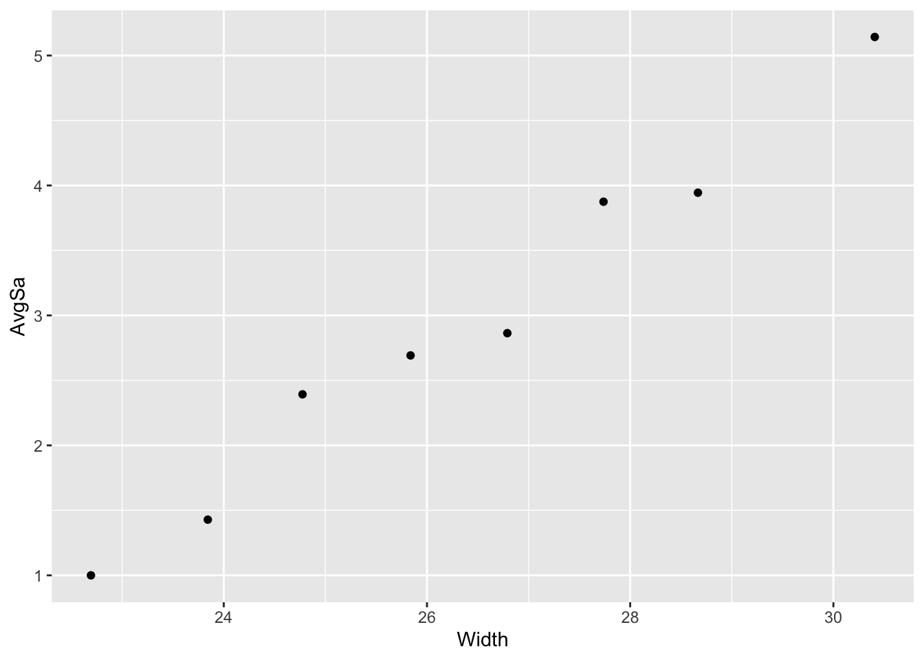
In this approach, we create 8 width groups and use the average width for the crabs in that group as the single representative value. While width is still treated as quantitative, this approach simplifies the model and allows all crabs with widths in a given group to be combined. The disadvantage is that differences in widths within a group are ignored, which provides less information overall. However, another advantage of using the grouped widths is that the saturated model would have 8 parameters, and the goodness of fit tests, based on \(8-2\) degrees of freedom, are more reliable.
To account for the fact that width groups will include different numbers of crabs, we will model the mean rate \(\mu/t\) of satellites per crab, where \(t\) is the number of crabs for a particular width group. This variable is treated much like another predictor in the data set. The difference is that this value is part of the response being modeled and not assigned a slope parameter of its own. We will see more details on the Poisson rate regression model in the next section.
The data, after being grouped into 8 intervals, is shown in the table below. Two columns to note in particular are “Cases”, the number of crabs with carapace widths in that interval, and “Width”, which now represents the average width for the crabs in that interval.
    Interval     Cases   Width   AvgSa    SDSa    VarSa
      =23.25        14  22.693  1.0000  1.6641   2.7692
 23.25-24.25        14  23.843  1.4286  2.9798   8.8792
 24.25-25.25        28  24.775  2.3929  2.5581   6.5439
 25.25-26.25        39  25.838  2.6923  3.3729  11.3765
 26.26-27.25        22  26.791  2.8636  2.6240   6.8854
 27.25-28.25        24  27.738  3.8750  2.9681   8.8096
 28.25-29.25        18  28.667  3.9444  4.1084  16.8790
      >29.25        14  30.407  5.1429  2.8785   8.2858
In this approach, each observation within a group is treated as if it has the same width.
In SAS, the Cases variable is input with the OFFSET option in the Model statement. We also create a variable LCASES=log(CASES) which takes the log of the number of cases within each grouping. This is our adjustment value \(t\) in the model that represents (abstractly) the measurement window, which in this case is the group of crabs with a similar width. So, \(t\) is effectively the number of crabs in the group, and we are fitting a model for the rate of satellites per crab, given carapace width.
data crabgrp;
input width cases SaTotal AvgSa;
lcases=log(cases);
cards;
22.69 14 14 1.00
23.84 14 20 1.428571
24.77 28 67 2.392857
25.84 39 105 2.692308
26.79 22 63 2.863636
27.74 24 93 3.875
28.67 18 71 3.944444
30.41 14 72 5.142857
;
proc genmod data=crabgrp order=data;
model SaTotal = width / dist=poisson link=log
 offset=lcases obstats residuals;
 output out=data3 p=pred;
run;
Here is the output. Note “Offset variable” under the “Model Information”.
The GENMOD Procedure
| Model Information | |
|---|---|
| Data Set | WORK.CRABGRP |
| Distribution | Poisson |
| Link Function | Log |
| Dependent Variable | SaTotal |
| Offset Variable | lcases |
| Number of Observations Read | 8 |
|---|---|
| Number of Observations Used | 8 |
| Parameter Information | |
|---|---|
| Parameter | Effect |
| Prm1 | Intercept |
| Prm2 | width |
| Criteria For Assessing Goodness Of Fit | |||
|---|---|---|---|
| Criterion | DF | Value | Value/DF |
| Deviance | 6 | 6.5168 | 1.0861 |
| Scaled Deviance | 6 | 6.5168 | 1.0861 |
| Pearson Chi-Square | 6 | 6.2470 | 1.0412 |
| Scaled Pearson X2 | 6 | 6.2470 | 1.0412 |
| Log Likelihood | 1652.1028 | ||
| Full Log Likelihood | -26.4809 | ||
| AIC (smaller is better) | 56.9617 | ||
| AICC (smaller is better) | 59.3617 | ||
| BIC (smaller is better) | 57.1206 | ||
| Algorithm converged. |
| Analysis Of Maximum Likelihood Parameter Estimates | |||||||
|---|---|---|---|---|---|---|---|
| Parameter | DF | Estimate | Standard Error |
Wald 95% Confidence Limits | Wald Chi-Square | Pr > ChiSq | |
| Intercept | 1 | -3.5355 | 0.5760 | -4.6645 | -2.4065 | 37.67 | <.0001 |
| width | 1 | 0.1727 | 0.0212 | 0.1311 | 0.2143 | 66.18 | <.0001 |
| Scale | 0 | 1.0000 | 0.0000 | 1.0000 | 1.0000 | ||
The scale parameter was held fixed.
Based on the Pearson and deviance goodness of fit statistics, this model clearly fits better than the earlier ones before grouping width. For example, the Value/DF for the deviance statistic now is 1.0861.
The estimated model is: \(\log (\hat{\mu}_i/t) = -3.535 + 0.1727\mbox{width}_i\)
For each 1-cm increase in carapace width, the mean number of satellites per crab is multiplied by \(\exp(0.1727)=1.1885.\)
See the full table…
The GENMOD Procedure
| Observation Statistics | |||||||||||||||||||||
|---|---|---|---|---|---|---|---|---|---|---|---|---|---|---|---|---|---|---|---|---|---|
| Observation | SaTotal | lcases | width | Predicted Value | Linear Predictor | Standard Error of the Linear Predictor | HessWgt | Lower | Upper | Raw Residual | Pearson Residual | Deviance Residual | Std Deviance Residual | Std Pearson Residual | Likelihood Residual | Leverage | CookD | DFBETA_Intercept | DFBETA_width | DFBETAS_Intercept | DFBETAS_width |
| 1 | 14 | 2.6390573 | 22.69 | 20.544353 | 3.0225861 | 0.1027001 | 20.544353 | 16.798637 | 25.12528 | -6.544353 | -1.443845 | -1.532938 | -1.732037 | -1.631372 | -1.710727 | 0.2166875 | 0.3681075 | -0.460663 | 0.0164188 | -0.799711 | 0.7733011 |
| 2 | 20 | 2.6390573 | 23.84 | 25.058503 | 3.2212132 | 0.0813848 | 25.058503 | 21.363886 | 29.392059 | -5.058503 | -1.010519 | -1.047745 | -1.14727 | -1.106509 | -1.140606 | 0.1659747 | 0.1218267 | -0.24937 | 0.008775 | -0.432905 | 0.4132908 |
| 3 | 67 | 3.3322045 | 24.77 | 58.849849 | 4.0749893 | 0.0657446 | 58.849849 | 51.734881 | 66.943322 | 8.1501507 | 1.062412 | 1.039205 | 1.2034817 | 1.2303572 | 1.2103746 | 0.2543698 | 0.2582108 | 0.3254536 | -0.011232 | 0.5649873 | -0.528993 |
| 4 | 105 | 3.6635616 | 25.84 | 98.608352 | 4.591156 | 0.0513763 | 98.608352 | 89.162468 | 109.05493 | 6.3916476 | 0.6436592 | 0.636887 | 0.740506 | 0.74838 | 0.7425635 | 0.2602795 | 0.0985341 | 0.144533 | -0.004711 | 0.2509092 | -0.221869 |
| 5 | 63 | 3.0910425 | 26.79 | 65.543892 | 4.18272 | 0.0448389 | 65.543892 | 60.029581 | 71.564747 | -2.543892 | -0.314219 | -0.316285 | -0.33944 | -0.337223 | -0.339149 | 0.1317776 | 0.0086301 | -0.015069 | 0.0003426 | -0.026159 | 0.0161352 |
| 6 | 93 | 3.1780538 | 27.74 | 84.252198 | 4.4338147 | 0.0468532 | 84.252198 | 76.859888 | 92.355494 | 8.7478019 | 0.9530338 | 0.9372168 | 1.0381222 | 1.0556422 | 1.0413848 | 0.1849521 | 0.1264386 | -0.069134 | 0.0033416 | -0.120017 | 0.1573828 |
| 7 | 71 | 2.8903718 | 28.67 | 74.1998 | 4.3067615 | 0.0562513 | 74.1998 | 66.454059 | 82.848368 | -3.1998 | -0.371468 | -0.374187 | -0.427757 | -0.424648 | -0.427029 | 0.2347839 | 0.0276639 | 0.0743554 | -0.003055 | 0.129081 | -0.143886 |
| 8 | 72 | 2.6390573 | 30.41 | 77.943052 | 4.3559785 | 0.0840923 | 77.943052 | 66.099465 | 91.908752 | -5.943052 | -0.673164 | -0.682002 | -1.017999 | -1.004806 | -1.010749 | 0.5511749 | 0.6199362 | 0.5164022 | -0.02006 | 0.8964738 | -0.944816 |
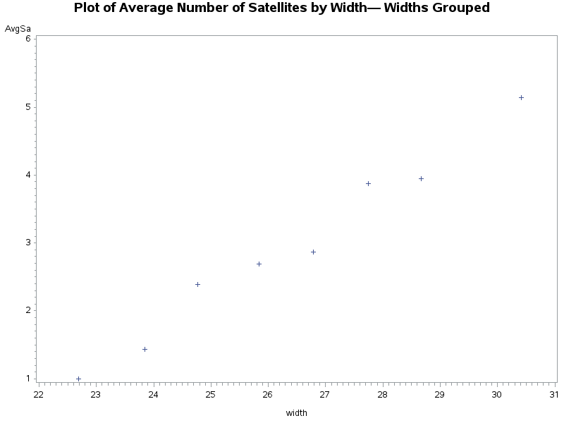
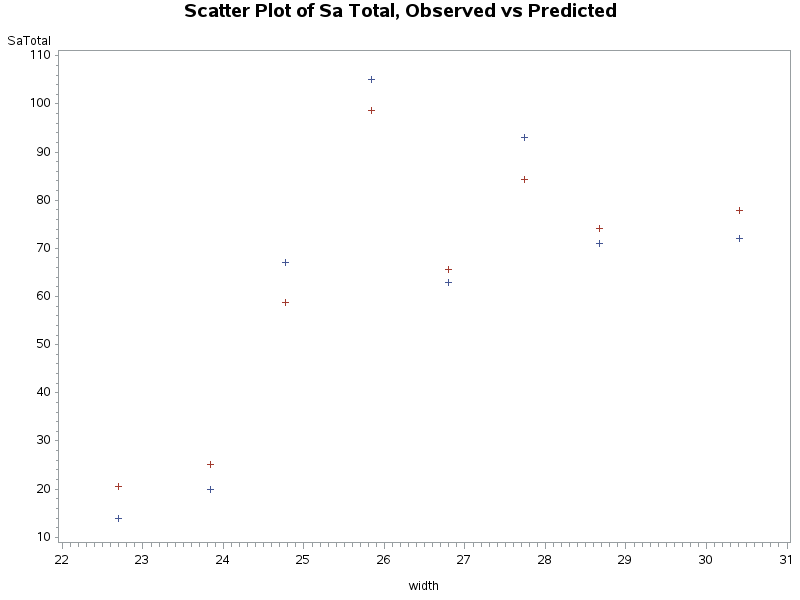
The residuals analysis indicates a good fit as well. From the table above we also see that the predicted values correspond a bit better to the observed counts in the SaTotal cells. Let’s compare the observed and fitted values in the plot below:
Plot of Number of Satellites by Width of Crab—All Data
Plot of Average Number of Satellites by Width— Widths Grouped
In R, the lcases variable is specified with the OFFSET option, which takes the log of the number of cases within each grouping. This is our adjustment value \(t\) in the model that represents (abstractly) the measurement window, which in this case is the group of crabs with similar width. So, \(t\) is effectively the number of crabs in the group, and we are fitting a model for the rate of satellites per crab, given carapace width.
# creating the 8 width groups
width.long = cut(hcrabs$W, breaks=c(0,seq(23.25, 29.25),Inf))

# summarizing per group
Cases = aggregate(hcrabs$W, by=list(W=width.long),length)$x
lcases = log(Cases)
Width = aggregate(hcrabs$W, by=list(W=width.long),mean)$x
AvgSa = aggregate(hcrabs$Sa, by=list(W=width.long),mean)$x
SdSa = aggregate(hcrabs$Sa, by=list(W=width.long),sd)$x
VarSa = aggregate(hcrabs$Sa, by=list(W=width.long),var)$x
SaTotal = aggregate(hcrabs$Sa, by=list(W=width.long),sum)$x
cbind(table(width.long), Width, AvgSa, SdSa, VarSa)

hcrabs.grp = data.frame(Width=Width, lcases=lcases, SaTotal=SaTotal)
model.grp = glm(SaTotal ~ Width, offset=lcases, family=poisson, data=hcrabs.grp)
summary(model.grp)
Here is the output. Note the offset = lcases under the model expression.
summary(model.grp)
Call:
glm(formula = SaTotal ~ Width, family = poisson, data = hcrabs.grp,
    offset = lcases)

Coefficients:
            Estimate Std. Error z value Pr(>|z|)
(Intercept) -3.54018    0.57658  -6.140 8.26e-10 ***
Width        0.17290    0.02125   8.135 4.11e-16 ***
---
Signif. codes:  0 '***' 0.001 '**' 0.01 '*' 0.05 '.' 0.1 ' ' 1

(Dispersion parameter for poisson family taken to be 1)

    Null deviance: 72.3772  on 7  degrees of freedom
Residual deviance:  6.5164  on 6  degrees of freedom
AIC: 56.961

Number of Fisher Scoring iterations: 4
Based on the Pearson and deviance goodness of fit statistics, this model clearly fits better than the earlier ones before grouping width. For example, the Value/DF for the deviance statistic now is 1.0861. The estimated model is:
\[ \log (\hat{\mu}_i/t)= -3.54 + 0.1729\mbox{width}_i \]
For each 1-cm increase in carapace width, the mean number of satellites per crab is multiplied by \(\exp(0.1729)=1.1887\).
rstandard(model.grp) 1 2 3 4 5 6 7
-1.6306867 -1.1066939 1.2246526 0.7527651 -0.3391852 1.0576113 -0.4229866
8
-1.0080897 predict.glm(model.grp, type="response", newdata=hcrabs.grp) 1 2 3 4 5 6 7 8
20.54097 25.05952 58.88382 98.57261 65.55897 84.23620 74.18733 77.96057 The residuals analysis indicates a good fit as well, and the predicted values correspond a bit better to the observed counts in the SaTotal cells. Let’s compare the observed and fitted values in the plot below:
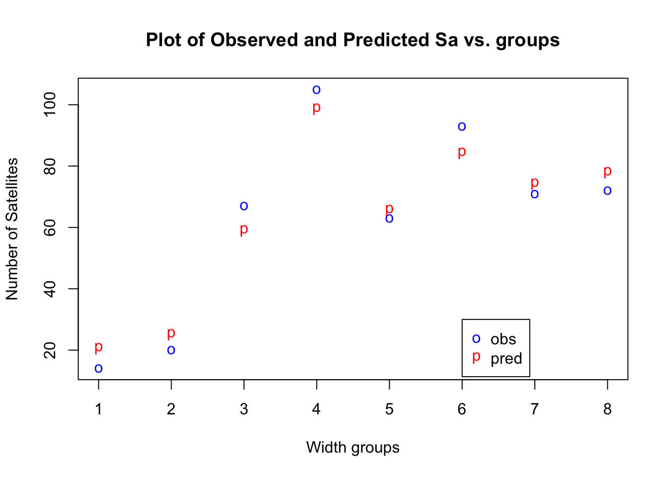
9.3 Modeling Rate Data
Example 9.2 (Lung Cancer Incidence) The table below summarizes the lung cancer incident counts (cases) per age group for four Danish cities from 1968 to 19711. Since it’s reasonable to assume that the expected count of lung cancer incidents is proportional to the population size, we would prefer to model the rate of incidents per capita.
city   age  pop cases
 Fredericia 40-54 3059    11
    Horsens 40-54 2879    13
    Kolding 40-54 3142     4
      Vejle 40-54 2520     5
 Fredericia 55-59  800    11
    Horsens 55-59 1083     6
    Kolding 55-59 1050     8
      Vejle 55-59  878     7
 Fredericia 60-64  710    11
    Horsens 60-64  923    15
    Kolding 60-64  895     7
      Vejle 60-64  839    10
 Fredericia 65-69  581    10
    Horsens 65-69  834    10
    Kolding 65-69  702    11
      Vejle 65-69  631    14
 Fredericia 70-74  509    11
    Horsens 70-74  634    12
    Kolding 70-74  535     9
      Vejle 70-74  539     8
 Fredericia   75+  605    10
    Horsens   75+  782     2
    Kolding   75+  659    12
      Vejle   75+  619     7
With \(Y_i\) the count of lung cancer incidents and \(t_i\) the population size for the \(i^{th}\) row in the data, the Poisson rate regression model would be
\[ \log \dfrac{\mu_i}{t_i}=\log \mu_i-\log t_i=\beta_0+\beta_1x_{1i}+\beta_2x_{2i}+\cdots \]
where \(Y_i\) has a Poisson distribution with mean \(E(Y_i)=\mu_i\), and \(x_1\), \(x_2\), etc. represent the (systematic) predictor set. Notice that by modeling the rate with population as the measurement size, population is not treated as another predictor, even though it is recorded in the data along with the other predictors. The main distinction the model is that no \(\beta\) coefficient is estimated for population size (it is assumed to be 1 by definition). Note also that population size is on the log scale to match the incident count.
By using an OFFSET option in the MODEL statement in GENMOD in SAS we specify an offset variable. The offset variable serves to normalize the fitted cell means per some space, grouping, or time interval to model the rates. In this case, population is the offset variable.
data cancer;
input city $ age $ pop cases;
lpop = log(pop);
cards;
 Fredericia 40-54 3059    11
    Horsens 40-54 2879    13
    Kolding 40-54 3142     4
      Vejle 40-54 2520     5
 Fredericia 55-59  800    11
    Horsens 55-59 1083     6
    Kolding 55-59 1050     8
      Vejle 55-59  878     7
 Fredericia 60-64  710    11
    Horsens 60-64  923    15
    Kolding 60-64  895     7
      Vejle 60-64  839    10
 Fredericia 65-69  581    10
    Horsens 65-69  834    10
    Kolding 65-69  702    11
      Vejle 65-69  631    14
 Fredericia 70-74  509    11
    Horsens 70-74  634    12
    Kolding 70-74  535     9
      Vejle 70-74  539     8
 Fredericia   75+  605    10
    Horsens   75+  782     2
    Kolding   75+  659    12
      Vejle   75+  619     7
; run;
proc genmod data=cancer;
class city(ref='Frederic') age(ref='40-54');
model cases = city age / dist=poi link=log offset=lpop type3;
run;
And, here is the output from the GENMOD procedure:
The GENMOD Procedure
| Model Information | |
|---|---|
| Data Set | WORK.CANCER |
| Distribution | Poisson |
| Link Function | Log |
| Dependent Variable | cases |
| Offset Variable | lpop |
| Number of Observations Read | 24 |
|---|---|
| Number of Observations Used | 24 |
| Class Level Information | ||
|---|---|---|
| Class | Levels | Values |
| city | 4 | Horsens Kolding Vejle Frederic |
| age | 6 | 55-59 60-64 65-69 70-74 75+ 40-54 |
| Criteria For Assessing Goodness Of Fit | |||
|---|---|---|---|
| Criterion | DF | Value | Value/DF |
| Deviance | 15 | 23.4475 | 1.5632 |
| Scaled Deviance | 15 | 23.4475 | 1.5632 |
| Pearson Chi-Square | 15 | 22.5616 | 1.5041 |
| Scaled Pearson X2 | 15 | 22.5616 | 1.5041 |
| Log Likelihood | 278.4530 | ||
| Full Log Likelihood | -59.9178 | ||
| AIC (smaller is better) | 137.8355 | ||
| AICC (smaller is better) | 150.6927 | ||
| BIC (smaller is better) | 148.4380 | ||
| Algorithm converged. |
By adding offset in the MODEL statement in GLM in R, we can specify an offset variable. The offset variable serves to normalize the fitted cell means per some space, grouping, or time interval to model the rates. In this case, population is the offset variable.
library(ISwR)
library(dplyr)
data(eba1977)
eba1977 = eba1977 %>% mutate(lpop = log(pop))
model = glm(cases ~ city + age, offset=lpop, family=poisson, data=eba1977)
summary(model)
anova(model, test='Chisq')
Here is the output we get:
summary(model)
Call:
glm(formula = cases ~ city + age, family = poisson, data = eba1977,
    offset = lpop)

Coefficients:
            Estimate Std. Error z value Pr(>|z|)
(Intercept)  -5.6321     0.2003 -28.125  < 2e-16 ***
cityHorsens  -0.3301     0.1815  -1.818   0.0690 .
cityKolding  -0.3715     0.1878  -1.978   0.0479 *
cityVejle    -0.2723     0.1879  -1.450   0.1472
age55-59      1.1010     0.2483   4.434 9.23e-06 ***
age60-64      1.5186     0.2316   6.556 5.53e-11 ***
age65-69      1.7677     0.2294   7.704 1.31e-14 ***
age70-74      1.8569     0.2353   7.891 3.00e-15 ***
age75+        1.4197     0.2503   5.672 1.41e-08 ***
---
Signif. codes:  0 '***' 0.001 '**' 0.01 '*' 0.05 '.' 0.1 ' ' 1

(Dispersion parameter for poisson family taken to be 1)

    Null deviance: 129.908  on 23  degrees of freedom
Residual deviance:  23.447  on 15  degrees of freedom
AIC: 137.84

Number of Fisher Scoring iterations: 5
The fitted model is
\[ \log\dfrac{\hat{\mu}}{t} = -5.6321-0.3301C_1-0.3715C_2-0.2723C_3 + 1.1010A_1+\cdots+1.4197A_5 \]
where \(C_1\), \(C_2\), and \(C_3\) are the indicators for cities Horsens, Kolding, and Vejle (Fredericia as baseline), and \(A_1,\ldots,A_5\) are the indicators for the last five age groups (40-54 as baseline).
Thus, for people in (baseline) age group 40-54 and in the city of Fredericia, the estimated average rate of lung cancer is
\[ \dfrac{\hat{\mu}}{t}=e^{-5.6321}=0.003581 \]
per person. For a group of 100 people in this category, the estimated average count of incidents would be \(100(0.003581)=0.3581\).
Does the overall model fit? From the deviance statistic 23.447 relative to a chi-square distribution with 15 degrees of freedom (the saturated model with city by age interactions would have 24 parameters), the p-value would be 0.0715, which is borderline. But the model with all interactions would require 24 parameters, which isn’t desirable either. Is there perhaps something else we can try?
Example 9.3 (Considering Age as Quantitative) Since age was originally recorded in six groups, we needed five separate indicator variables to model it as a categorical predictor. We may also consider treating it as quantitative variable if we assign a numeric value, say the midpoint, to each group.
The following code creates a quantitative variable for age from the midpoint of each age group. It also creates an empirical rate variable for use in plotting. Note that this empirical rate is the sample ratio of observed counts to population size \(Y/t\), not to be confused with the population rate \(\mu/t\), which is estimated from the model.
data cancer;
set cancer;
if age='40-54' then age_mid=47;
if age='55-59' then age_mid=57;
if age='60-64' then age_mid=62;
if age='65-69' then age_mid=67;
if age='70-74' then age_mid=72;
if age='75+' then age_mid=75;
e_rate = cases/pop;
run;
proc sgplot data=cancer;
reg y=e_rate x=age_mid / group=city;
run;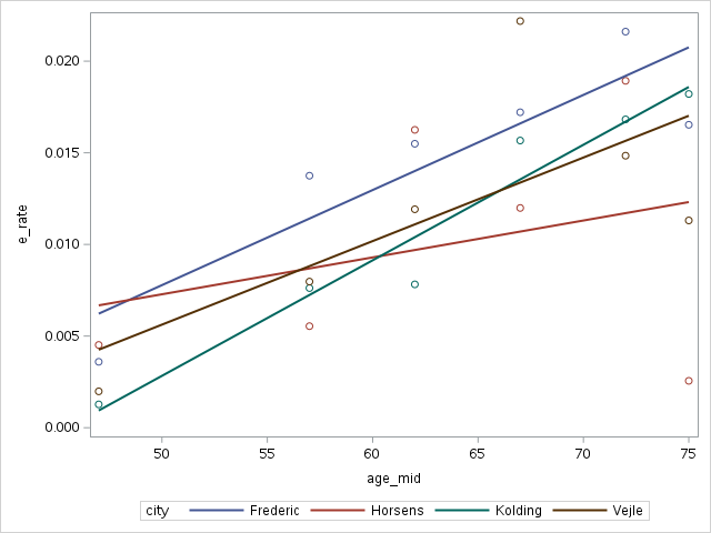
With age treated as quantitative, we no longer include it in the CLASS statement.
proc genmod data=cancer;
class city;
model cases = age_mid / dist=poi link=log offset=lpop type3;
run;
The interpretation of the slope for age is now the increase in the rate of lung cancer (per capita) for each 1-year increase in age, provided city is held fixed.
The GENMOD Procedure
| Model Information | |
|---|---|
| Data Set | WORK.CANCER |
| Distribution | Poisson |
| Link Function | Log |
| Dependent Variable | cases |
| Offset Variable | lpop |
| Number of Observations Read | 24 |
|---|---|
| Number of Observations Used | 24 |
| Class Level Information | ||
|---|---|---|
| Class | Levels | Values |
| city | 4 | Horsens Kolding Vejle Frederic |
| Criteria For Assessing Goodness Of Fit | |||
|---|---|---|---|
| Criterion | DF | Value | Value/DF |
| Deviance | 19 | 46.4483 | 2.4446 |
| Scaled Deviance | 19 | 46.4483 | 2.4446 |
| Pearson Chi-Square | 19 | 41.4714 | 2.1827 |
| Scaled Pearson X2 | 19 | 41.4714 | 2.1827 |
| Log Likelihood | 266.9526 | ||
| Full Log Likelihood | -71.4182 | ||
| AIC (smaller is better) | 152.8363 | ||
| AICC (smaller is better) | 156.1696 | ||
| BIC (smaller is better) | 158.7266 | ||
| Algorithm converged. |
| Analysis Of Maximum Likelihood Parameter Estimates | ||||||||
|---|---|---|---|---|---|---|---|---|
| Parameter | DF | Estimate | Standard Error |
Wald 95% Confidence Limits | Wald Chi-Square | Pr > ChiSq | ||
| Intercept | 1 | -7.9822 | 0.4311 | -8.8271 | -7.1373 | 342.89 | <.0001 | |
| city | Horsens | 1 | -0.3053 | 0.1814 | -0.6609 | 0.0503 | 2.83 | 0.0924 |
| city | Kolding | 1 | -0.3503 | 0.1877 | -0.7182 | 0.0176 | 3.48 | 0.0620 |
| city | Vejle | 1 | -0.2460 | 0.1878 | -0.6140 | 0.1220 | 1.72 | 0.1901 |
| city | Frederic | 0 | 0.0000 | 0.0000 | 0.0000 | 0.0000 | . | . |
| age_mid | 1 | 0.0568 | 0.0065 | 0.0440 | 0.0696 | 75.62 | <.0001 | |
| Scale | 0 | 1.0000 | 0.0000 | 1.0000 | 1.0000 | |||
The scale parameter was held fixed.
| LR Statistics For Type 3 Analysis | |||
|---|---|---|---|
| Source | DF | Chi-Square | Pr > ChiSq |
| city | 3 | 4.25 | 0.2357 |
| age_mid | 1 | 80.07 | <.0001 |
library(dplyr)
eba1977 = eba1977 %>% mutate(
  age.mid = rep(c(47,57,62,67,72,75), each=4),
  e.rate = cases/pop)
ggplot(eba1977, aes(x=age.mid, y=e.rate, color=city)) +
  geom_point() + geom_smooth(method='lm', se=FALSE)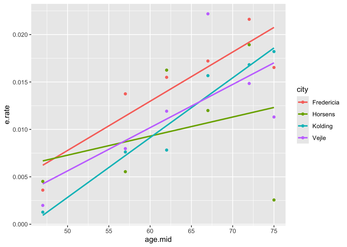
The plot generated shows increasing trends between age and lung cancer rates for each city. There is also some evidence for a city effect as well as for city by age interaction, but the significance of these is doubtful, given the relatively small data set.
As we have seen before when comparing model fits with a predictor as categorical or quantitative, the benefit of treating age as quantitative is that only a single slope parameter is needed to model a linear relationship between age and the cancer rate. The tradeoff is that if this linear relationship is not accurate, the lack of fit overall may still increase.
model = glm(cases ~ city + age.mid, offset=lpop, family=poisson, data=eba1977)
summary(model)
anova(model, test='Chisq')
The interpretation of the slope for age is now the increase in the log rate of lung cancer (per capita) for each 1-year increase in age, provided city is held fixed.
summary(model)
Call:
glm(formula = cases ~ city + age.mid, family = poisson, data = eba1977,
    offset = lpop)

Coefficients:
             Estimate Std. Error z value Pr(>|z|)
(Intercept) -7.982221   0.431070 -18.517   <2e-16 ***
cityHorsens -0.305279   0.181423  -1.683   0.0924 .
cityKolding -0.350278   0.187705  -1.866   0.0620 .
cityVejle   -0.246016   0.187769  -1.310   0.1901
age.mid      0.056759   0.006527   8.696   <2e-16 ***
---
Signif. codes:  0 '***' 0.001 '**' 0.01 '*' 0.05 '.' 0.1 ' ' 1

(Dispersion parameter for poisson family taken to be 1)

    Null deviance: 129.908  on 23  degrees of freedom
Residual deviance:  46.448  on 19  degrees of freedom
AIC: 152.84

Number of Fisher Scoring iterations: 5
9.4 Lesson Summary
In this lesson, we showed how the generalized linear model can be applied to count data, using the Poisson distribution with the log link. Compared with the logistic regression model, two differences we noted are the option to use the negative binomial distribution as an alternate random component when correcting for overdispersion and the use of an offset to adjust for observations collected over different windows of time, space, etc. Much of the properties otherwise are the same (parameter estimation, deviance tests for model comparisons, etc.).
One other common characteristic between logistic and Poisson regression that we change for the log-linear model coming up is the distinction between explanatory and response variables. The log-linear model makes no such distinction and instead treats all variables of interest together jointly. This allows greater flexibility in what types of associations can be fit and estimated, but one restriction in this model is that it applies only to categorical variables.
Source: E.B. Andersen (1977), Multiplicative Poisson models with unequal cell rates, Scandinavian Journal of Statistics, 4:153–158.↩︎