5: Three-Way Tables: Types of Independence
5: Three-Way Tables: Types of IndependenceOverview
This lesson spells out analysis techniques for three-way tables which is a representative analysis of any K-way table. We begin with the structure of a three-way table, and its corresponding joint, marginal and conditional distributions. In particular, we distinguish between a marginal and a conditional odds ratio. We then consider how to extend the goodness-of-fit tests that we saw in the previous lessons. Now there will be a variety of models of independence and associations (see the list below). It is natural to think about using the tests we developed for two-way tables on three-way tables. Many of the models we discuss in this lesson correspond to a particular choice of how to turn a three-way table into a two-way table.
The concept of conditional independence is very important and it is the basis for many statistical models (e.g., latent class models, factor analysis, item response models, graphical models, etc.). With respect to conditional independence models, we will see more on Cochran-Mantel-Haenszel (CMH) statistics, and describe the phenomenon known as Simpson's paradox. We will also learn about a model of homogeneous associations. In a later lesson on Log-Linear models, we will learn how to answer the same questions but via models instead of goodness-of-fit tests.
Each of the models described in this lesson will be given a mathematical formulation, e.g., a formula for the expected counts when possible. If that's not your "cup of tea", you can skip those paragraphs and focus on conceptual understanding and how we do the relevant tests in SAS and/or R.
A three-way contingency table is a cross-classification of observations by the levels of three categorical variables. More generally, k-way contingency tables classify observations by levels of k categorical variables. Levels may be ordinal or nominal.
Lesson 5 Code Files
SAS Files
Useful Links
- SAS source on stratified tables
- R: Cochran-Mantel-Haenszel Chi-Squared Test for Count Data
- R: Breslow-Day test: function for the class, breslowday.test()
5.1 - Notation and Structure
5.1 - Notation and StructureA three-way contingency table is a cross-classification of observations by the levels of three categorical variables. Suppose that we have three categorical variables, \(X\), \(Y\), and \(Z\), where
\(X\) takes possible values \(1,2,\ldots,I\)
\(Y\) takes possible values \(1,2,\ldots,J\)
\(Z\) takes possible values \(1,2,\ldots,K\)
If we collect the triplet \((X,Y,Z)\) for each individual in a sample of size \(n\), then the data can be summarized as a three-dimensional table. Let \(n_{ijk}\) be the number of units for which \(X = i\), \(Y = j\), and \(Z = k\). Then the vector of cell counts \((n_{111}, n_{112}, \dots , n_{IJK})\) can be arranged in a table whose dimensions are \(I \times J \times K\). Geometrically, we can think of this as a cube. For example, the Rubik’s cube is a \(3 \times 3 \times 3\) table.
Example: Berkeley Admissions
The table below lists graduate admissions information for the six largest departments at U.C. Berkeley in the fall of 1973.
| Dept. | Males admitted | Males rejected | Females admitted | Females rejected |
|---|---|---|---|---|
| A | 512 | 313 | 89 | 19 |
| B | 353 | 207 | 17 | 8 |
| C | 120 | 205 | 202 | 391 |
| D | 138 | 279 | 131 | 244 |
| E | 53 | 138 | 94 | 299 |
| F | 22 | 351 | 24 | 317 |
Although it's arranged in a \(6\times 4\) table to easily view on this page, we can imagine this in three dimensions as a \(2\times2\times6\) table, where \(X =\) sex (1 = male, 2 = female), \(Y =\) admission status (1 = admitted, 2 = rejected), and \(Z =\) department (1 = A, 2 = B, . . ., 6 = F), in which case \(n_{112}= 353\) corresponds to the number of males admitted to department B.
Possible questions of interest here would be whether admission rates differ by sex or among departments. As we'll see, however, these relationships can be measured in different ways.
Partial Tables
To display three-way tables, we typically use a set of two-way tables. These are referred to as partial tables. There are three ways to do this:
- Consider \(I\), \(Y\times Z\) tables for each level of \(X\)
- Consider \(J\), \(X\times Z\) tables for each level of \(Y\)
- Consider \(K\), \(X\times Y\) tables for each level of \(Z\)
For example, we could look at the two-way (partial) table between sex and admission status for each department in the Berkeley data. This representation corresponds to a conditional distribution because the department is fixed within each table. For the first two departments, we have
Department A
| Admission status | |||
|---|---|---|---|
| Admitted | Rejected | ||
| Sex | Male | 512 | 313 |
| Female | 89 | 19 | |
Department B
| Admission status | |||
|---|---|---|---|
| Admitted | Rejected | ||
| Sex | Male | 353 | 207 |
| Female | 17 | 8 | |
Marginal Tables
As before, we will use "+" to indicate summation over a subscript; for example in the expression below we sum over \(k\),
\(n_{ij+}=\sum\limits_{k=1}^K n_{ijk}\).
Then the vector of counts \((n_{11+}, n_{12+}, \dots, n_{IJ+})\) can be arranged into a table of \(I\times J\) dimensions, referred to as the marginal table of \(X\) and \(Y\). There are three possible two-way marginal tables resulting from one three-way table. Essentially, by summing over one variable, we ignore its association with each of the other variables. This idea can even extend to the marginal table of a single variable by summing over both of the other variables.
In the Berkeley admission example, the table below is the marginal one between sex and admission status, obtained by summing over the six departments. If we had observed only this table, we would not know anything about the departments.
| Admitted | Rejected | Total | |
| Male | 1198 | 1493 | 2691 |
| Female | 557 | 1278 | 1835 |
| Total | 1755 | 2771 | 4526 |
Joint Distribution
If the \(n\) individuals in the sample are independent and identically distributed (IID), that is if they are a random sample, then the vector of cell counts \( ({n_{111}, n_{112}, \dots, n_{IJK}})\) has a multinomial distribution with index \(n = n_{+++}\) and vector of probabilities \(\pi=(\pi_{111},\pi_{112},\ldots,\pi_{IJK})\), where
\(\pi_{ijk} = P(X = i, Y = j, Z = k)\)
That is, \(\pi_{ijk}\) is the joint probability that a randomly selected individual falls in the \((i, j, k)\) cell of the contingency table. Under the unrestricted (saturated) multinomial model, there are no constraints on \(\pi\) other than \(\sum\limits_{i=1}^I \sum\limits_{j=1}^J\sum\limits_{k=1}^K\pi_{ijk}= 1\), and the maximum likelihood (ML) estimates are the sample proportions: \(\hat{\pi}_{ijk}=n_{ijk}/n\). The saturated model always fits the data perfectly, and the expected frequency of the \((i, j, k)\) cell \(\mu_{ijk}=n\pi_{ijk}\) is estimated with \(n\hat{\pi}_{ijk}=n_{ijk}\), the observed frequency of the \((i, j, k)\) cell for all \(i\), \(j\), and \(k\).
Question: This model yields \(X^2 = G^2 = 0\) with zero degrees of freedom. Why?
Fitting a saturated model might not reveal any special structure that may exist in the relationships among the variables. To investigate these relationships, we propose simpler models and perform tests to see whether these simpler models fit the data by comparing them to the saturated model---that is the observed data---as we did in the previous lessons. These new models will depend on marginal and conditional distributions.
Conditional Distributions
The conditional distribution is a subset of variables given another mutually exclusive subset of variables. For example, the conditional distribution of \(X\) and \(Y\), given \(Z\), is \({\pi_{ij|k}} = \pi_{ijk} / \pi_{++k}\), such that \(\sum_{ij} \pi{ij|k} = 1\). Intuitively, we're asking how the joint distribution of \(X\) and \(Y\) change as the levels of \(Z\) change.
We can also consider the conditional distribution of one variable given the other two. For example, \({\pi_{j|ik}} = \pi_{ijk} / \pi_{i+k}\), such that \(\sum_j \pi_{j|ik} = 1\). This is the conditional distribution of \(Y\), given both \(X\) and \(Z\). Intuitively, we're asking how the distribution of \(Y\) changes as the levels of either \(X\) or \(Z\) changes.
| Department B | |||
|---|---|---|---|
| Admission status | |||
| Admitted | Rejected | ||
| Sex | Male | 353/585=0.6034 | 207/585=0.3538 |
| Female | 17/585=0.0291 | 8/585=0.0137 | |
Notice that these proportions necessarily sum to one.
Marginal associations and conditional associations can be very different! In the next section, we define and study the marginal and conditional odds-ratios to help us understand a potential difference in these associations and their impact on statistical inference.
Sampling Schemes
What are some ways of generating three-way (or higher) tables of counts? We essentially have the same sampling schemes as what we saw for two-way tables:
- Poisson unrestricted sampling – nothing is fixed, each cell is a Poisson random variable with a rate \(\mu_{ijk}\)
- Multinomial sampling with fixed total sample size \(n\)
With higher tables, since we have more "total" sample sizes to fix, we have additional ways to think of sampling such as:
- Stratified sampling where we have the product-multinomial sampling with fixed sample size for each partial table, e.g. \(n_{++k}\)
- Product-Multinomial sampling within each partial table, e.g. fix \(n_{i+k}\), that is fix the rows within each partial table.
Next, let's define marginal and conditional odds-ratios.
5.2 - Marginal and Conditional Odds Ratios
5.2 - Marginal and Conditional Odds RatiosMarginal Odds Ratios
Marginal Odds Ratios
Marginal odds ratios are odds ratios between two variables in the marginal table and can be used to test for marginal independence between two variables while ignoring the third.
For example, for the \(XY\) margin, where \( \mu_{ij+}\) denotes the expected count of individuals with \(X=i\) and \(Y=j\) in the marginal table obtained by summing over \(Z\), the marginal odds ratio is
\(\theta_{XY}=\dfrac{\mu_{11+}\mu_{22+}}{\mu_{12+}\mu_{21+}}\)
And the estimate of this from the admission data would be
\(\hat{\theta}_{XY}=\dfrac{1198\cdot1278}{1493\cdot557}=1.84\)
Thus, if we aggregate values over all departments, the odds that a male is admitted are an estimated 1.84 times as high as the odds that a female is admitted. And if we were to calculate a suitable confidence interval (e.g., 95%), it would not include 1, indicating that the odds for males is significantly higher.
Conditional Odds Ratios
Conditional Odds Ratios
Conditional odds ratios are odds ratios between two variables for fixed levels of the third variable and allow us to test for conditional independence of two variables, given the third.
For example, for the fixed level \(Z=k\), the conditional odds ratio between \(X\) and \(Y\) is
\(\theta_{XY(k)}=\dfrac {\mu_{11k}\mu_{22k}}{\mu_{12k}\mu_{21k}}\)
There are as many such conditional odds ratios as there are levels of the conditional variable, and each can be estimated from the corresponding conditional or partial table between \(X\) and \(Y\), given \(Z=k\). For the first two departments of the admission data, the estimated conditional odds ratios between sex and admission status would be
\(\hat{\theta}_{XY(Z=1)}=\dfrac{512\cdot19}{89\cdot313}=0.35\)
and
\(\hat{\theta}_{XY(Z=2)}=\dfrac{353\cdot8}{17\cdot207}=0.80\)
That is, if we restrict our attention to Department A only, the odds that a male is admitted are an estimated 0.35 times as high as the odds that a female is admitted. Or, equivalently, the odds that a female is admitted are an estimated \(1/0.35=2.86\) times that for males. Likewise, the odds of being admitted are higher for females if we restrict our attention to Department B.
We are calculating the odds ratios for the various partial tables of the larger table and can use them to test the conditional independence of \(X\) and \(Y\), given \(Z\). If \(\theta_{XY(k)} \ne 1\) for at least one level of \(Z\) (at least one \(k\)), it follows that \(X\) and \(Y\) are conditionally associated. We will learn more about this, but for now, let's utilize our knowledge of two-way tables to do some preliminary analysis.
Using what we know about \(2\times2\) tables and tests for association, we can compare the marginal and conditional odds ratios for our example and measure evidence for their significance. What do they tell us about the relationships among these variables?
Let's look at using the SAS program file berkeley.sas (Full output: berkely SAS Output.
                                        /* Analysis of a 3-way table Berkeley Admissions data using PROC FREQ */
                                        options nocenter nodate nonumber linesize=72;
                                        data berkeley;
                                           input D $ S $ A $ count;
                                           cards;
                                        DeptA  Male    Reject  313
                                        DeptA  Male    Accept  512
                                        DeptA  Female  Reject   19
                                        DeptA  Female  Accept   89
                                        DeptB  Male    Reject  207
                                        DeptB  Male    Accept  353
                                        DeptB  Female  Reject    8
                                        DeptB  Female  Accept   17
                                        DeptC  Male    Reject  205
                                        DeptC  Male    Accept  120
                                        DeptC  Female  Reject  391
                                        DeptC  Female  Accept  202
                                        DeptD  Male    Reject  279
                                        DeptD  Male    Accept  138
                                        DeptD  Female  Reject  244
                                        DeptD  Female  Accept  131
                                        DeptE  Male    Reject  138
                                        DeptE  Male    Accept   53
                                        DeptE  Female  Reject  299
                                        DeptE  Female  Accept   94
                                        DeptF  Male    Reject  351
                                        DeptF  Male    Accept   22
                                        DeptF  Female  Reject  317
                                        DeptF  Female  Accept   24
                                        ;
                                        /*analysis of the three-way table including CMH test*/
                                        proc freq data=berkeley order=data;
                                        weight count;
                                        tables D*S*A/ cmh chisq relrisk expected nocol norow;
                                        tables S*A/chisq relrisk;
                                        run;
The tables command is where we can specify which variables to tabulate; those that are omitted are summed over (marginalized). For example,
tables S*A/chisq all nocol nopct;will create a marginal table of sex and admission status, and compute all the relevant statistics for this \(2\times2\) table (see below). To get the partial tables and analyses of sex and admissions status for each department, we can run the following line:
tables D*S*A /chisq cmh nocol nopct;We will discuss the CMH option later. In PROC FREQ, the partial tables will be created given the levels of the first variable you specify when creating a three-way table. We can see the full output of this program in berkeley SAS Output.
Statistical Inference
Marginal Independence
Let's first look at the marginal table of sex and admission status, while ignoring departments. As we calculated earlier, the point estimate of the odds-ratio is 1.84. That is, the odds of admission for males are an estimated 1.84 times as high as that for females, and it can be shown to be statistically significant based on the 95% confidence interval or a chi-square test of independence. However, keep in mind that we ignored the department information here. A more precise statement would be to say that sex and admission status are marginally associated.
|
| ||||||||||||||||||||||||
Statistics for Table of S by A
Statistic | DF | Value | Prob |
|---|---|---|---|
Chi-Square | 1 | 92.6704 | <.0001 |
Likelihood Ratio Chi-Square | 1 | 93.9232 | <.0001 |
Continuity Adj. Chi-Square | 1 | 92.0733 | <.0001 |
Mantel-Haenszel Chi-Square | 1 | 92.6499 | <.0001 |
Phi Coefficient | -0.1431 | ||
Contingency Coefficient | 0.1416 | ||
Cramer's V | -0.1431 |
Odds Ratio and Relative Risks | |||
|---|---|---|---|
Statistic | Value | 95% Confidence Limits | |
Odds Ratio | 0.5423 | 0.4785 | 0.6147 |
Relative Risk (Column 1) | 0.7961 | 0.7608 | 0.8330 |
Relative Risk (Column 2) | 1.4679 | 1.3535 | 1.5919 |
Conditional Independence
Now consider the point estimates of odds ratios when we control for the department, which uses conditional odds-ratios (see Sec. 5.2.) Given that the individuals are applying to Department A, the odds of male admission are 0.35 times as high as the odds of female admission, and this is also significant at the 0.05 level (its 95% CI (0.2087, 0.5843) does not include the value 1). Other conditional odds ratios (Department B, C, etc.) are not significant, but it's interesting to note, nevertheless, that these conditional relationships do not have to be in the same direction as the marginal one. When they disagree, we have an example of Simpson's Paradox.
|
| ||||||||||||||||||||||||||||
Statistics for Table 1 of S by A
Controlling for D=DeptA
Statistic | DF | Value | Prob |
|---|---|---|---|
Chi-Square | 1 | 17.2480 | <.0001 |
Likelihood Ratio Chi-Square | 1 | 19.0540 | <.0001 |
Continuity Adj. Chi-Square | 1 | 16.3718 | <.0001 |
Mantel-Haenszel Chi-Square | 1 | 17.2295 | <.0001 |
Phi Coefficient | 0.1360 | ||
Contingency Coefficient | 0.1347 | ||
Cramer's V | 0.1360 |
Odds Ratio and Relative Risks | |||
|---|---|---|---|
Statistic | Value | 95% Confidence Limits | |
Odds Ratio | 2.8636 | 1.7112 | 4.7921 |
Relative Risk (Column 1) | 2.1566 | 1.4206 | 3.2737 |
Relative Risk (Column 2) | 0.7531 | 0.6799 | 0.8341 |
R users should open the berkeley.R file and its corresponding output file berkeley.out. R will calculate the partial tables by the levels of the last variable in the array.
#### Berkeley Admissions Example: a 2x2x6 table
                #### let X=sex, Y=admission status, Z=department
                library(survival)
                library(vcd)
                #### data available as an array in R
                admit <- UCBAdmissions
                dimnames(admit) <- list(
                Admit=c("Admitted","Rejected"),
                Sex=c("Male","Female"),
                Dept=c("A","B","C","D","E","F"))
                admit
                #### create a flat contingency table
                ftable(admit, row.vars=c("Dept","Sex"), col.vars="Admit")
                ### conditional odds ratios
                XY.Z <- oddsratio(admit) # log scale
                exp(XY.Z$coef)
                exp(confint(XY.Z))
                plot(XY.Z)
                ### Cochran-Mantel-Haenszel test of conditional independence
                mantelhaen.test(admit)
                mantelhaen.test(admit, correct=FALSE)
                ### marginal tables and odds ratios
                XY <- margin.table(admit, c(2,1))
                ZY <- margin.table(admit, c(3,1))
                XZ <- margin.table(admit, c(2,3))
                oddsratio(XY, log=FALSE)
                exp(confint(oddsratio(XY)))
                chisq.test(XY, correct=FALSE)
                #source(file.choose()) # choose breslowday.test_.R
                breslowday.test(admit)
We can also use ftable() function, e.g.,
ftable(admit, row.vars=c("Dept","Sex"), col.vars="Admit")to create flat tables. In this case, R essentially combines the departments and sexes into 12-row categories, resulting in a \(12\times2\) representation of the original \(2\times2\times6\) table. To create a marginal table, we can use margin.table() to
margin.table(admit, c(2,1))This function creates a marginal table of the second (sex) and the first (admission status) variables from the original array, which in this case puts the sexes as the rows and admission status groups as the columns.
Statistical Inference
Marginal Independence
Let's first look at the marginal table of sex and admission status, while ignoring departments. As we calculated earlier, the point estimate of the odds-ratio is 1.84. That is, the odds of admission for males are an estimated 1.84 times as high as that for females, and it can be shown to be statistically significant based on the 95% confidence interval or a chi-square test of independence. However, keep in mind that we ignored the department information here. A more precise statement would be to say that sex and admission status are marginally associated.
XY <- margin.table(admit, c(2,1))
                                                                                chisq.test(XY, correct=FALSE)
Pearson's Chi-squared test
>data:  XY
                                                                                X-squared = 92.205, df = 1, p-value < 2.2e-16
Conditional Independence
Now consider the point estimates of odds ratios when we control for the department, which uses conditional odds-ratios (see Sec. 5.2.) Given that the individuals are applying to Department A, the odds of male admission are 0.35 times as high as the odds of female admission, and this is also significant at the 0.05 level (its 95% CI (0.2087, 0.5843) does not include the value 1). Other conditional odds ratios (Department B, C, etc.) are not significant, but it's interesting to note, nevertheless, that these conditional relationships do not have to be in the same direction as the marginal one. When they disagree, we have an example of Simpson's Paradox.
XY.Z <- oddsratio(admit) # log scale
                                                                                exp(XY.Z$coef)
A B C D E F
0.3492120 0.8025007 1.1330596 0.9212838 1.2216312 0.8278727
2.5 % 97.5 %
A 0.2086756 0.5843954
B 0.3403815 1.8920166
C 0.8545328 1.5023696
D 0.6863345 1.2366620
E 0.8250748 1.8087848
F 0.4552059 1.5056335Simpson’s paradox
Simpson's paradox is the phenomenon that a pair of variables can have marginal association and partial (conditional) associations in opposite direction. Another way to think about this is that the nature and direction of association changes due to the presence or absence of a third (possibly confounding) variable.
In the simplest example, consider three binary variables, \(X\), \(Y\), \(Z\). In the marginal table where we are ignoring the presence of \(Z,\) let
\(P(Y = 1|X = 1) < P(Y = 1|X = 2)\)
In the partial table, after we account for the presence of variable \(Z,\) let
\(P(Y = 1|X = 1,Z = 1) > P(Y = 1|X = 2, Z = 1)\) and
\(P(Y = 1|X = 1,Z = 2) > P(Y = 1|X = 2, Z = 2)\)
In terms of odds ratios, marginal odds \(\theta_{XY} < 1\), and partial odds \(\theta_{XY(Z=1)} > 1\) and \(\theta_{XY(Z=2)} > 1\).
These associations can also be captured in terms of models. Next, we explore more on different independence and association concepts that capture relationships between three categorical variables.
Additional Resources (optional)
Here is Dr. Jason Morton with a quick video explanation of what this paradox involves.
In addition, for those of you that would like to delve a little deeper into this, here is a link to "Algebraic geometry of 2 × 2 contingency tables" by Slavkovic and Fienberg. On page 17 of this document is a diagram of this paradox as well.
5.3 - Models of Independence and Associations in 3-Way Tables
5.3 - Models of Independence and Associations in 3-Way TablesFor multinomial sampling and a two-dimensional table, only independence of row and column is of interest. With three-dimensional tables, there are at least eight models of interest. In the next sections of this lesson, we are going to look at different models of independence and dependence that can capture relationships between variables in a three-way table. Please note that these concepts extend to any number of categorical variables (e.g., \(k\)-way table), and are not unique to categorical data only. But we will consider their mathematical and graphical representation and interpretations within the context of categorical data and links to odd-ratios, marginal, and partial tables. In the later lessons, we will see different ways of fitting these models (e.g., log-linear models, logistic regression, etc.).
Recall that independence means no association, but there are many types of association that might exist among variables. Here are the types of independence and associations relationships (i.e., models) that we will consider.
- Mutual independence -- all variables are independent from each other, denoted \((X,Y,Z)\) or \(X\perp\!\!\perp Y \perp\!\!\perp Z\).
- Joint independence -- two variables are jointly independent of the third, denoted \((XY,Z)\) or \(X Y \perp\!\!\perp Z\).
- Marginal independence -- two variables are independent while ignoring the third, e.g., \(\theta_{XY}=1\), denoted \((X,Y)\).
- Conditional independence -- two variables are independent given the third, e.g., \(\theta_{XY(Z=k)}=1\), for all \(k=1,2,\ldots,K\), denoted \((XZ, YZ)\) or \(X \perp\!\!\perp Y | Z\).
- Homogeneous associations -- conditional (partial) odds-ratios don't depend on the value of the third variable, denoted \((XY, XZ, YZ)\).
Before we look at the details, here is a summary of the relationships among these models:
- Mutual independence implies joint independence, i.e., all variables are independent of each other.
- Joint independence implies marginal independence, i.e., one variable is independent of the other two.
- Marginal independence does NOT imply joint independence.
- Marginal independence does NOT imply conditional independence.
- Conditional independence does NOT imply marginal independence.
It is worth noting that a minimum of three variables is required for all the above types of independence to be defined.
5.3.1 - Mutual (Complete) Independence
5.3.1 - Mutual (Complete) IndependenceThe simplest model that one might propose is that ALL variables are independent of one another. Graphically, if we have three random variables, \(X\), \(Y\), and \(Z\) we can express this model as:
In this graph, the lack of connections between the nodes indicates no relationships exist among \(X\), \(Y\), and \(Z{,}\) or there is mutual independence. In the notation of log-linear models, which will learn about later as well, this model is expressed as (\(X\), \(Y\), \(Z\)). We will use this notation from here on. The notation indicates which aspects of the data we consider in the model. In this case, the independence model means we care only about the marginals totals \(n_{i++}, n_{+j+}, n_{++k}\) for each variable separately, and these pieces of information will be sufficient to fit a model and compute the expected counts. Alternatively, as we will see later on, we could keep track of the number of times some joint outcome of two variables occurs.
In terms of odds ratios, the model (\(X\), \(Y\), \(Z\)) implies that if we look at the marginal tables \(X \times Y\), \(X \times Z\) , and \(Y\times Z\) , then all of the odds ratios in these marginal tables are equal to 1. In other words, mutual independence implies marginal independence (i.e., there is independence in the marginal tables). All variables are really independent of one another.
Under this model the following must hold:
\(P(X=i,Y=j,Z=k)=P(X=i)P(Y=j)P(Z=k)\)
for all \(i, j, k\). That is, the joint probabilities are the product of the marginal probabilities. This is a simple extension from the model of independence in two-way tables where it was assumed:
\(P(X=i,Y=j)=P(X=i)P(Y=j)\)
We denote the marginal probabilities
\(\pi_{i++} = P(X = i), i = 1, 2, \ldots , I \)
\(\pi_{+j+} = P(Y = j), j = 1, 2, \ldots, J\)
\(\pi_{++k} = P(Z = k), k = 1, 2, \ldots , K\)
so that \(\pi_{ijk} = [\pi_{i++}\pi_{+j+}\pi_{++k}\) for all \(i, j, k\). Then the unknown parameters of the model of independence are
\(\pi_{i++} = (\pi_{1++}, \pi_{2++},\ldots, \pi_{I++})\)
\(\pi_{+j+} = (\pi_{+1+}, \pi_{+2+},\ldots , \pi_{+J+})\)
\(\pi_{++k} = (\pi_{++1}, \pi_{++2},\ldots , \pi_{++K})\)
Under the assumption that the model of independence is true, once we know the marginal probability values, we have enough information to estimate all unknown cell probabilities. Because each of the marginal probability vectors must add up to one, the number of free parameters in the model is \((I − 1) + (J − 1) + (K −I )\). This is exactly like the two-way table, but now one more set of additional parameter(s) needs to be taken care of for the additional random variable.
Consider the Berkeley admissions example, where under the independence model, the number of free parameters is \((2-1) + (2-1) + (6-1) = 7\), and the marginal distributions are
\((n_{1++}, n_{2++}, \ldots , n_{I++}) \sim Mult(n, \pi_{i++})\)
\((n_{+1+}, n_{+2+}, \ldots , n_{+J+}) \sim Mult(n, \pi_{+j+})\)
\((n_{++1}, n_{++2}, \ldots , n_{++K}) \sim Mult(n, \pi_{++k})\)
and these three vectors are mutually independent. Thus, the three parameter vectors \(\pi_{i++}, \pi_{+j+}\), and \(\pi_{++k}\) can be estimated independently of one another. The ML estimates are the sample proportions in the margins of the table,
\(\hat{\pi}_{i++}=p_{i++}=n_{i++}/n,\quad i=1,2,\ldots,I\)
\(\hat{\pi}_{+j+}=p_{+j+}=n_{+j+}/n,\quad j=1,2,\ldots,J\)
\(\hat{\pi}_{++k}=p_{++k}=n_{++k}/n,\quad k=1,2,\ldots,K\)
It then follows that the estimates of the expected cell counts are
\(E(n_{ijk})=n\hat{\pi}_{i++}\hat{\pi}_{+j+}\hat{\pi}_{++k}=\dfrac{n_{i++}n_{+j+}n_{++k}}{n^2}\)
Compare this to a two-way table, where the expected counts were:
\(E(n_{ij})=n_{i+}n_{+j}/n\).
For the Berkeley admission example, the marginal tables, i.e., counts are \(X=(2691, 1835)\) (for sex), \(Y=(1755 2771)\) (for admission status), and \(Z=(933, 585, 918, 792, 584, 714)\) (for department). The first (estimated) expected count would be \(E(n_{111})=2691(1755)(933)/4526^2=215.1015\), for example. Then, we compare these expected counts with the corresponding observed counts. That is, 215.1015 would be compared with \(n_{111}=512\) and so on.
Chi-Squared Test of Independence
The hypothesis of independence can be tested using the general method described earlier:
\(H_0 \colon\) the independence model is true vs. \(H_A \colon\) the saturated model is true
In other words, we can check directly \(H_0\colon \pi_{ijk} = \pi_{i++}\pi_{+j+}\pi_{++k}\) for all \(i, j, k\), vs. \(H_A\colon\) the saturated model
- Estimate the unknown parameters of the independence model, i.e.., the marginal probabilities.
- Calculate estimated cell probabilities and expected cell frequencies \(E_{ijk}=E(n_{ijk})\) under the model of independence.
- Calculate \(X^2\) and/or \(G^2\) by comparing the expected and observed values, and compare them to the appropriate chi-square distribution.
\(X^2=\sum\limits_i \sum\limits_j \sum\limits_k \dfrac{(E_{ijk}-n_{ijk})^2}{E_{ijk}}\)
\(G^2=2\sum\limits_i \sum\limits_j \sum\limits_k n_{ijk} \log\left(\dfrac{n_{ijk}}{E_{ijk}}\right)\)
The degrees of freedom (DF) for this test are \(\nu = (IJK − 1) − [ (I − 1) + (J − 1) + (K − 1)]\). As before, this is a difference between the number of free parameters for the saturated model \((IJK-1)\) and the number of free parameters in the current model of independence, \((I-1)+(J-1)+(K-1)\). In the case of the Berkeley data, we have \(23-7 = 16\) degrees of freedom for the mutual independence test.
Recall that we also said that mutual independence implies marginal independence. So, if we reject marginal independence for any pair of variables, we can immediately reject mutual independence overall. For example, recall the significant result when testing for the marginal association between sex and admission status (\(X^2=92.205\)). Since we rejected marginal independence in that case, it would expect to reject mutual (complete) independence as well.
Example: Boys Scouts and Juvenile Delinquency
This is a \(2 \times 2 \times 3\) table. It classifies \(n = 800\) boys according to socioeconomic status (S), whether they participated in boy scouts (B), and whether they have been labeled as a juvenile delinquent (D):
| Socioeconomic status | Boy scout | Delinquent | |
|---|---|---|---|
| Yes | No | ||
| Low | Yes | 11 | 43 |
| No | 42 | 169 | |
| Medium | Yes | 14 | 104 |
| No | 20 | 132 | |
| High | Yes | 8 | 196 |
| No | 2 | 59 | |
To fit the mutual independence model, we need to find the marginal totals for B,
\(n_{1++} = 11 + 43 + 14 + 104 + 8 + 196 = 376\)
\(n_{2++} = 42 + 169 + 20 + 132 + 2 + 59 = 424\)
for D,
\(n_{+1+} = 11 + 42 + 14 + 20 + 8 + 2 = 97\)
\(n_{+2+} = 43 + 169 + 104 + 132 + 196 + 59 = 703\)
and for S,
\(n_{++1} = 11 + 43 + 42 + 169 = 265\)
\(n_{++2} = 14 + 104 + 20 + 132 = 270\)
\(n_{++3} = 8 + 196 + 2 + 59 = 265\)
Next, we calculate the expected counts for each cell,
\(E_{ijk}=\dfrac{n_{i++}n_{+j+}n_{++k}}{n^2}\)
and then calculate the chi-square statistic. The degrees of freedom for this test are \((2\times 2\times 3-1)-[(2-1)+(2-1)+(3-1)]=7\) so the \(p\)-value can be found as \(P(\chi^2_7 \geq X^2)\) and \(P(\chi^2_7 \geq G^2)\).
In SAS, we can use the following lines of code:
data answers;
a1=1-probchi(218.6622,7);
;
proc print data=answers;
run;
In R, we can use 1-pchisq(218.6622, 7).
The p-values are essentially zero, indicating that the mutual independence model does not fit. Remember, in order for the chi-squared approximation to work well, the \(E_{ijk}\) needs to be sufficiently large. Sufficiently large means that most of them (e.g., about at least 80%) should be at least five, and none should be less than one. We should examine the \(E_{ijk}\) to see if they are large enough.
Fortunately, both R and SAS will give the expected counts, (in parentheses) and the observed counts:
| Socioeconomic status | Boy scout | Delinquent | |
|---|---|---|---|
| Yes | No | ||
| Low | Yes | 11 (15.102) |
43 (109.448) |
| No | 42 (17.030) |
169 (123.420) |
|
| Medium | Yes | 14 (15.387 ) |
104 |
| No | 20 (17.351) |
132 (125.749) |
|
| High | Yes |
8 |
196 (109.448) |
| No | 2 (17.030) |
59 |
|
Here, the expected counts are sufficiently large for the chi-square approximation to work well, and thus we must conclude that the variables B (boys scout), D (delinquent), and S (socioeconomic status) are not mutually independent.
There is no single function or a call in SAS nor R that will directly test the mutual independence model; see will see how to fit this model via a log-linear model. However, we can test this by relying on our understanding of two-way tables, and of marginal and partial tables and related odds ratios. For mutual independence to hold, all of the tests for independence in marginal tables must hold. Thus, we can do the analysis of all two-way marginal tables using the chi-squared test of independence in each. Alternatively, we can consider the odds-ratios in each two-way table. In this case, for example, the estimated odds ratio for the \(B \times D\) table, is 0.542, and it is not equal to 1; i.e., 1 is not in covered by the 95% odds-ratio confidence interval, (0.347, 0.845). Therefore, we have sufficient evidence to reject the null hypothesis that boy scout status and delinquent status are independent of one another and thus that \(B\), \(D\), and \(S\) are not mutually independent.
The following SAS or R code supports the above analysis by testing independence of two-way marginal tables. Again, we will see later in the course that this is done more efficiently via log-linear models.
Here we will use the SAS code found in the program boys.sas as shown below.
data boys;
input SES $scout $ delinquent $ count @@;
datalines;
low yes yes 11 low yes no 43
low no yes 42 low no no 169
med yes yes 14 med yes no 104
med no yes 20 med no no 132
high yes yes 8 high yes no 196
high no yes 2 high no no 59
;
proc freq;
 weight count;
 tables SES;
 tables scout;
 tables delinquent;
 tables SES*scout/all nocol nopct;
 tables SES*delinquent/all nocol nopct;
 tables scout*delinquent/all nocol nopct;
 tables SES*scout*delinquent/chisq cmh expected nocol nopct;
run;
The output for this program can be found in this file: boys.lst.
For R, we will use the R program file boys.R to create contingency tables and carry out the test of mutual independence.
#### Test of conditional independence
#### Use of oddsratio(), confit() from {vcd}
#### Cochran-Mantel-Haenszel test
#### Also testing via Log-linear models
############################################

#### Input the table

deliquent=c("no","yes")
scout=c("no", "yes")
SES=c("low", "med","high")
table=expand.grid(deliquent=deliquent,scout=scout,SES=SES)
count=c(169,42,43,11,132,20,104,14,59,2,196,8)
table=cbind(table,count=count)
table
temp=xtabs(count~deliquent+scout+SES,table)
temp

#### Create "flat" contigency tables

ftable(temp)

#### Let's see how we can create various subtables
#### One-way Table SES

Frequency=as.vector(margin.table(temp,3))
CumFrequency=cumsum(Frequency)
cbind(SES,Frequency=Frequency,Percentage=Frequency/sum(Frequency),CumFrequency=CumFrequency,CumPercentage=CumFrequency/sum(Frequency))

#### One-way Table scout

Frequency=as.vector(margin.table(temp,2))
CumFrequency=cumsum(Frequency)
cbind(scout,Frequency=Frequency,Percentage=Frequency/sum(Frequency),CumFrequency=CumFrequency,CumPercentage=CumFrequency/sum(Frequency))

#### One-way Table deliquent

Frequency=as.vector(margin.table(temp,1))
CumFrequency=cumsum(Frequency)
cbind(deliquent,Frequency=Frequency,Percentage=Frequency/sum(Frequency),CumFrequency=CumFrequency,CumPercentage=CumFrequency/sum(Frequency))

#### Test the Mutual Independence, step by step
#### compute the expected frequencies

E=array(NA,dim(temp))
for (i in 1:dim(temp)[1]) {
for (j in 1:dim(temp)[2]) {
for (k in 1:dim(temp)[3]) {
E[i,j,k]=(margin.table(temp,3)[k]*margin.table(temp,2)[j]*margin.table(temp,1))[i]/(sum(temp))^2
}}}
E

#### compute the X^2, and G^2

df=(length(temp)-1)-(sum(dim(temp))-3)
X2=sum((temp-E)^2/E)
X2
1-pchisq(X2,df)
G2=2*sum(temp*log(temp/E))
G2
1-pchisq(G2,df)


#### Test for Mutual indpendence (and other models) by considering analysis of all two-way tables
#### Two-way Table SES*scout
#### This is a test of Marginal Independence for SES and Scout

SES_Scout=margin.table(temp,c(3,2))
result=chisq.test(SES_Scout)
result
result$expected
result=chisq.test(SES_Scout,correct = FALSE)
result
SES_Scout=list(Frequency=SES_Scout,RowPercentage=prop.table(SES_Scout,2))


#### Two-way Table SES*deliquent
#### temp=xtabs(count~scout+SES+deliquent,table)
#### SES_deliquent=addmargins(temp)[1:2,1:3,3]
#### This is a test of Marginal Independence for SES and deliquent status

SES_deliquent=margin.table(temp,c(3,1))
result=chisq.test(SES_deliquent)
result
result$expected
result=chisq.test(SES_deliquent,correct = FALSE)
result
SES_deliquent=list(Frequency=SES_deliquent,RowPercentage=prop.table(SES_deliquent,2))

#### Two-way Table deliquent*scout
#### This is a test of Marginal Independence for Deliquent status and the Scout status

deliquent_scout=margin.table(temp,c(1,2))
result=chisq.test(deliquent_scout)
result$expected
result=chisq.test(deliquent_scout,correct = FALSE)
result
deliquent_scout1=list(Frequency=deliquent_scout,RowPercentage=prop.table(deliquent_scout,1))

#### compute the log(oddsraio), oddsratio and its 95% CI using {vcd} package

lor=oddsratio(deliquent_scout)
lor
OR=exp(lor)
OR
OR=oddsratio(deliquent_scout, log=FALSE)
OR
CI=exp(confint(lor))
CI
CI=confint(OR)
CI


#### Table of deliquent*scout at different level of SES

temp

#### Test for Joint Independence of (D,BS)
#### creating 6x2 table, BS x D

SESscout_deliquent=ftable(temp, row.vars=c(3,2))
result=chisq.test(SESscout_deliquent)
result

#### Test for Marginal Independence (see above analysis of two-way tables)

#### Test for conditional independence
#### To get partial tables of DB for each level of S

temp[,,1]
chisq.test(temp[,,1], correct=FALSE)
temp[,,2]
chisq.test(temp[,,2], correct=FALSE)
temp[,,3]
chisq.test(temp[,,3], correct=FALSE)
X2=sum(chisq.test(temp[,,1], correct=FALSE)$statistic+chisq.test(temp[,,2], correct=FALSE)$statistic+chisq.test(temp[,,3], correct=FALSE)$statistic)
1-pchisq(X2,df=3)

#### Cochran-Mantel-Haenszel test

mantelhaen.test(temp)
mantelhaen.test(temp,correct=FALSE)

#### Breslow-Day test
#### make sure to first source/run breslowday.test_.R

breslowday.test(temp)

################################################################
#### Log-linear Models
#### Let's see how we would do this via Log_linear models
#### We will look at the details later in the course
#### test of conditional independence
#### via loglinear model, but the object has to be a table!

is.table(temp)  #### to check if table
temp<-as.table(temp) #### to save as table
temp.condind<-loglin(temp, list(c(1,3), c(2,3)), fit=TRUE, param=TRUE) #### fit the cond.indep. model
temp.condind
1-pchisq(temp.condind$lrt, temp.condind$df)

#### There is no way to do Breslow-Day stats in R;
#### you need to write your own function or fit the homogeneous association model
#### to test for identity of odds-ratios

#### test of homogenous association model

temp.hom<-loglin(temp, list(c(1,3), c(2,3), c(1,2)), fit=TRUE, param=TRUE)
temp.hom
1-pchisq(temp.hom$lrt, temp.hom$df)


#### Here is how to do the same but with the glm() function in R
#### test of conditional independence
#### via loglinear mode, but using glm() funcion
#### the object now needs to be dataframe

temp.data<-as.data.frame(temp)
temp.data
temp.condind<-glm(temp.data$Freq~temp.data$scout*temp.data$SES+temp.data$deliquent*temp.data$SES, family=poisson())
summary(temp.condind)
fitted(temp.condind)

#### test of homogenous association model

temp.hom<-glm(temp.data$Freq~temp.data$scout*temp.data$SES+temp.data$deliquent*temp.data$SES+temp.data$scout*temp.data$deliquent, family=poisson())
summary(temp.hom)
fitted(temp.hom)
The output file, boys.out contains the results for these procedures.
5.3.2 - Joint Independence
5.3.2 - Joint IndependenceThe joint independence model implies that two variables are jointly independent of a third. For example, let's suggest that C is jointly independent of \(X\) and \(Y\). In the log-linear notation, this model is denoted as (\(XY\), \(Z{)}\). Here is a graphical representation of this model:
which indicates that \(X\) and \(Y\) are jointly independent of \(Z\). The line linking \(X\) and \(Y\) indicates that \(X\) and \(Y\) are possibly related, but not necessarily so. Therefore, the model of complete independence is a special case of this one.
For three variables, three different joint independence models may be considered. If the model of complete independence (\(X\), \(Y\), \(Z\)) fits a data set, then the model (\(XY\), \(Z\)) will also fit, as will (\(XZ\), \(Y\)) and (\(YZ\), \(X\)). In that case, we will prefer to use (\(X\), \(Y\), \(Z\)) because it is more parsimonious; our goal is to find the simplest model that fits the data. Note that joint independence does not imply mutual independence. This is one of the reasons why we start with the overall model of mutual independence before we collapse and look at models of joint independence.
Assuming that the (\(XY\), \(Z\)) model holds, the cell probabilities would be equal to the product of the marginal probabilities from the \(XY\) margin and the \(Z\) margin:
\(\pi_{ijk} = P(X = i,Y= j) P(Z = k) = \pi_{ij}+ \pi_{++k},\)
where \(\sum_i \sum_j \pi_{ij+} = 1\) and \(\sum_k \pi_{++k} = 1\). Thus if we know the counts in the \(XY\) table and the \(Z\) table, we can compute the expected counts in the \(XYZ\) table. The number of free parameters, that is the number of unknown parameters that we need to estimate is \((IJ − 1) + (K − 1)\), and their ML estimates are \(\hat{\pi}_{ij+}=n_{ij+}/n\), and \(\hat{\pi}_{++k}=n_{++k}/n\). The estimated expected cell frequencies are:
\(\hat{E}_{ijk}=\dfrac{n_{ij+}n_{++k}}{n}\) (1)
Notice the similarity between this formula and the one for the model of independence in a two-way table, \(\hat{E}_{ij}=n_{i+}n_{+j}/n\). If we view \(X\) and \(Y\) as a single categorical variable with \(IJ\) levels, then the goodness-of-fit test for (\(XY\), \(Z\)) is equivalent to the test of independence between the combined variable \(XY\) and \(Z\). The implication of this is that you can re-write the 3-way table as a 2-way table and do its analysis.
To determine the degrees of freedom in order to evaluate this model and to construct the chi-squared and deviance statistics, we need to find the number of free parameters in the saturated model and subtract from this the number of free parameters in the new model. We take the difference of the number of parameters we fit in the saturated model and the number of parameters we fit in the assumed model: DF = \((IJK-1)-[(IJ-1)+(K-1)]\), and this is equal to \((IJ-1)(K-1)\), which ties in the statement above that this is equivalent to the test of independence in a two-way table with a variable (\(XY\)) vs. variable (\(Z\)).
Example: Boy Scouts and Juvenile Delinquency
Going back to the boy scout example, let’s think of juvenile delinquency D as the response variable, and the other two — boy scout status B and socioeconomic status S—as explanatory variables or predictors. Therefore, it would be useful to test the null hypothesis that D is independent of B and S, or (D, BS).
Because we used \(i\), \(j\), and \(k\) to index B, D, and S, respectively, the estimated expected cell counts under the model "B and S are independent of D" are a slight rearrangement of (1) above,
\(E_{ijk}=\dfrac{n_{i+k}n_{+j+}}{n}\)
We can calculate the \(E_{ijk}\)s by this formula or in SAS or R by entering the data as a two-way table with one dimension corresponding to D and the other dimension corresponding to B \(\times\) S. In fact, looking at the original table, we see that the data are already arranged in the correct fashion; the two columns correspond to the two levels of D, and the six rows correspond to the six levels of a new combined variable B \(\times\) S. To test the hypothesis "D is independent of B and S," we simply enter the data as a \(6\times 2\) matrix, where we have combined the socioeconomic status (SES) with scout status, essentially collapsing the 3-way table into a 2-way table.
The SAS code for this example is: boys.sas.
Here is the SAS code shown below:
data boys;
input SES $scout $ delinquent $ count @@;
datalines;
low yes yes 11 low yes no 43
low no yes 42 low no no 169
med yes yes 14 med yes no 104
med no yes 20 med no no 132
high yes yes 8 high yes no 196
high no yes 2 high no no 59
;
proc freq;
 weight count;
 tables SES;
 tables scout;
 tables delinquent;
 tables SES*scout/all nocol nopct;
 tables SES*delinquent/all nocol nopct;
 tables scout*delinquent/all nocol nopct;
 tables SES*scout*delinquent/chisq cmh expected nocol nopct;
run;
Expected counts are printed below in the SAS output as the second entry in each cell:
The FREQ Procedure
|
|
||||||||||||||||||||||||||||||||||||||||
Statistics for Table of SES_scout by delinquent
| Statistic | DF | Value | Prob |
|---|---|---|---|
| Chi-Square | 5 | 32.9576 | <.0001 |
| Likelihood Ratio Chi-Square | 5 | 36.4147 | <.0001 |
| Mantel-Haenszel Chi-Square | 1 | 5.5204 | 0.0188 |
| Phi Coefficient | 0.2030 | ||
| Contingency Coefficient | 0.1989 | ||
| Cramer's V | 0.2030 |
The SAS output from this program is essentially evaluating a 2-way table, which we have already done before.
We will use the R code boys.R and look for the "Joint Independence" comment heading, and use of the ftable() function as shown below.
#### Test for Joint Independence of (D,BS)
#### creating 6x2 table, BS X D

SESscout_delinquent=ftable(temp, row.vars=c(3,2))
results=chisq.test(SESscout_delinquent)
result
Here is the output that R gives us:
Pearson's Chi-squared test

  data: SESscout_deliquent
  X-squared = 32.958, df = 5, p-value = 3.837e-06
Our conclusions are based on the following evidence: the chi-squared statistics values (e.g., \(X^2, G^2\)) are very large (e.g., \(X^2=32.9576, df=5\)), and the p-value is essentially zero, indicating that B and S are not independent of D. The expected cell counts are all greater than five, so this p-value is reliable and our hypothesis does not hold - we reject this model of joint independence.
Notice that we can also test for the other joint independence models, e.g., (BD, S), that is, the scout status and delinquency are jointly independent of the SES, and this involves analyzing a \(4\times3\) table, and (SD,B), that is the SES and Delinquency are jointly independent of the Boy's Scout status, and this involves analyzing a \(6\times2\) table. These are just additional analyses of two-way tables.
It is worth noting that while many different varieties of models are possible, one must keep in mind the interpretation of the models. For example, assuming delinquency to be the response, the model (D, BS) would have a natural interpretation; if the model holds, it means that B and S cannot predict D. But if the model does not hold, either B or S may be associated with D. However, (BD, S) and (SD, B) may not render themselves to easy interpretation, although statistically, we can perform the tests of independence.
5.3.3 - Marginal Independence
5.3.3 - Marginal IndependenceMarginal independence has already been discussed before. Variables \(X\) and \(Y\) are marginally independent if:
\(\pi_{ij+}=\pi_{i++}\pi_{+j+}\)
They are marginally independent if they are independent within the marginal table. In other words, we consider the relationship between \(X\) and \(Y\) only and completely ignore \(Z\). Controlling for, or adjusting for different levels of \(Z\) would involve looking at the partial tables.
We saw this already with the Berkeley admission example. Recall from the marginal table between sex and admission status, where the estimated odds-ratio was 1.84. We also had significant evidence that the corresponding odds-ratio in the population was different from 1, which indicates a marginal relationship between sex and admission status.
Question: How would you test the model of marginal independence between scouting and SES status in the boy-scout example? See the files boys.sas (boys.lst) or boys.R (boys.out) to answer this question. Hint: look for the chi-square statistic \(X^2=172.2\).
Recall, that joint independence implies marginal, but not the other way around. For example, if the model (\(XY\), \(Z\)) holds, it will imply \(X\) independent of \(Z\), and \(Y\) independent of \(Z\). But if \(X\) is independent of \(Z\) , and \(Y\) is independent of \(Z\), this will NOT necessarily imply that \(X\) and \(Y\) are jointly independent of \(Z\).
If \(X\) is independent of \(Z\) and \(Y\) is independent of \(Z\) we can’t tell if there is an association between \(X\) and \(Y\) or not; it could go either way, that is in our graphical representation there could be a link between \(X\) and \(Y\) but there may not be one either.
For example, let’s consider a \(2\times2\times2\) table.
The following \(XZ\) table has \(X\) independent of \(Z\) because each cell count is equal to the product of the corresponding margins divided by the total (e.g., \(n_{11}=2=8(5/20)\), or equivalently, OR = 1)
| C=1 | C=2 | Total | |
|---|---|---|---|
| A=1 | 2 | 6 | 8 |
| A=2 | 3 | 9 | 12 |
| Total | 5 | 15 | 20 |
The following \(YZ\) table has \(Y\) independent of \(Z\) because each cell count is equal to the product of the corresponding margins divided by the total (e.g., \(n_{11}=2=8(5/20)\)).
|
C=1 |
C=2 |
Total |
|
|---|---|---|---|
|
B=1 |
2 |
6 |
8 |
|
B=2 |
3 |
9 |
12 |
|
Total |
5 |
15 |
20 |
The following \(XY\) table is consistent with the above two tables, but here \(X\) and \(Y\) are NOT independent because all cell counts are not equal to the product of the corresponding margins divided by the total (e.g., \(n_{11}=2\)), whereas \(8(8/20)=16/5\)). Or you can see this via the odds ratio, which is not equal to 1.
| B=1 | B=2 | Total | |
|---|---|---|---|
| A=1 | 2 | 6 | 8 |
| A=2 | 6 | 6 | 12 |
| Total | 8 | 12 | 20 |
Furthermore, the following \(XY\times Z\) table is consistent with the above tables but here \(X\) and \(Y\) are NOT jointly independent of \(Z\) because all cell counts are not equal to the product of the corresponding margins divided by the total (e.g., \(n_{11}=1\), whereas \(2(5/20)=0.5\)).
| C=1 | C=2 | Total | |
|---|---|---|---|
| A=1, B=1 | 1 | 1 | 2 |
| A=1, B=2 | 1 | 5 | 6 |
| A=2, B=1 | 1 | 5 | 6 |
| A=2, B=2 | 2 | 4 | 6 |
| Total | 5 | 15 | 20 |
Other marginal independence models in a three-way table would be, \((X,Y)\) while ignoring \(Z\), and \((Y,Z)\), ignoring any information on \(X\).
5.3.4 - Conditional Independence
5.3.4 - Conditional IndependenceThe concept of conditional independence is very important and it is the basis for many statistical models (e.g., latent class models, factor analysis, item response models, graphical models, etc.).
There are three possible conditional independence models with three random variables: (\(XY\), \(XZ\)), (\(XY\), \(YZ\)), and (\(XZ\), \(YZ\)). Consider the model (\(XY\), \(XZ\)),
which means that \(Y\) and \(Z\) are conditionally independent given \(X\). In mathematical terms, the model (\(XY\), \(XZ\)) means that the conditional probability of \(Y\) and \(Z\), given \(X\) equals the product of conditional probabilities of \(Y\) given \(X\) and \(Z\), given \(X\):
\(P(Y=j,Z=k|X=i)=P(Y=j|X=i) \times P(Z=k|X=i)\)
In terms of odds-ratios, this model implies that if we look at the partial tables, that is \(Y\times Z\) tables at each level of \(X = 1, \ldots , I\), that the odds-ratios in these tables should not significantly differ from 1. Tying this back to 2-way tables, we can test in each of the partial \(Y\times Z\) tables at each level of \(X\) to see if independence holds.
\(H_0\colon \theta_{YZ\left(X=i\right)} = 1\) for all i
vs.
\(H_0\colon\) at least one \(\theta_{YZ\left(X=i\right)} \ne 1\)
- Recall, \((XY, XZ)\) implies that \(P(Y,Z| X)=P(Y|X)P(Z|X)\).
- If \((X,Y,Z)\) holds then we know that \(P(X, Y, Z)= P(X) P(Y) P(Z)\), and we also know that the mutual independence implies that \(P(Y|X)=P(Y)\) and \(P(Z|X)=P(Z)\).
- Thus from the probability properties, \(P(Y,Z|X)=P(X,Y,Z)/P(X)\) and from (2) above, \(P(Y,Z|X)=P(X,Y,Z)/P(X) = P(X)P(Y)P(Z)/P(X)= P(Y)P(Z)=P(Y|X)P(Z|X)\), which equals the expression in (1)
Intuitively, \((XY, XZ)\) means that any relationship that may exist between \(Y\) and \(Z\) can be explained by \(X\) . In other words, \(Y\) and \(Z\) may appear to be related if \(X\) is not considered (e.g. only look at the marginal table \(Y\times Z\), but if one could control for \(X\) by holding it constant (i.e. by looking at subsets of the data having identical values of \(X\), that is looking at partial tables \(Y\times Z\) for each level of \(X\)), then any apparent relationship between \(Y\) and \(Z\) would disappear (remember Simpson's paradox?). Marginal and conditional associations can be different!
Under the conditional independence model, the cell probabilities can be written as
\begin{align} \pi_{ijk} &= P(X=i) P(Y=j,Z=k|X=i)\\ &= P(X=i)P(Y=j|X=i)P(Z=k|X=i)\\ &= \pi_{i++}\pi_{j|i}\pi_{k|i}\\ \end{align}
where \(\sum_i \pi_{i++} = 1, \sum_j \pi_{j | i} = 1\) for each i, and \(\sum_k \pi_{k | i} = 1\) for each \(i\). The number of free parameters is \((I − 1) + I (J − 1) + I (K − 1)\).
The ML estimates of these parameters are
\(\hat{\pi}_{i++}=n_{i++}/n\)
\(\hat{\pi}_{j|i}=n_{ij+}/n_{i++}\)
\(\hat{\pi}_{k|i}=n_{i+k}/n_{i++}\)
and the estimated expected frequencies are
\(\hat{E}_{ijk}=\dfrac{n_{ij+}n_{i+k}}{n_{i++}}.\)
Notice again the similarity to the formula for independence in a two-way table.
The test for conditional independence of \(Y\) and \(Z\) given \(X\) is equivalent to separating the table by levels of \(X = 1, \ldots , I\) and testing for independence within each level.
There are two ways we can test for conditional independence:
- The overall \(X^2\) or \(G^2 \)statistics can be found by summing the individual test statistics for \(YZ\) independence across the levels of \(X\). The total degrees of freedom for this test must be \(I (J − 1)(K − 1)\). See the example below, and we’ll see more on this again when we look at log-linear models. Note, if we can reject independence in one of the partial tables, then we can reject the conditional independence and don't need to run the full analysis.
- Cochran-Mantel-Haenszel Test (using option CMH in PROC FREQ/ TABLES/ in SAS and mantelhaen.test in R). This test produces the Mantel-Haenszel statistic also known as the "average partial association" statistic.
Example: Boy Scouts and Juvenile Delinquency
Let us return to the table that classifies \(n = 800\) boys by scout status B, juvenile delinquency D, and socioeconomic status S. We already found that the models of mutual independence (D, B, S) and joint independence (D, BS) did not fit. Thus we know that either B or S (or both) are related to D. Let us temporarily ignore S and see whether B and D are related (marginal independence). Ignoring S means that we classify individuals only by the variables B and D; in other words, we form a two-way table for B \(\times\) D, the same table that we would get by collapsing (i.e. adding) over the levels of S.
| Boy scout | Delinquent | |
|---|---|---|
| Yes | No | |
| Yes | 33 | 343 |
| No | 64 | 360 |
The \(X^2\) test for this marginal independence demonstrates that a relationship between B and D does exist. Expected counts are printed below the observed counts:
| Delinquent=Yes | Delinquent=No | Total | |
|---|---|---|---|
| Boy Scout=Yes | 33 45.59 |
343 330.41 |
376 |
| Boy Scout=No | 64 51.41 |
360 372.59 |
424 |
| Total | 97 | 703 | 800 |
\(X^2 = 3.477 + 0.480 + 3.083 + 0.425 = 7.465\), where each value in the sum is a contribution (squared Pearson residual) of each cell to the overall Pearson \(X^2\) statistic. With df = 1, the p-value=1- PROBCHI(7.465,1)=0.006 in SAS or in R p-value=1-pchisq(7.465,1)=0.006, rejecting the marginal independence of B and D. This would also be consistent with the chi-square test of independence in the \(2\times2\) table.
The odds ratio of \((33 \cdot360)/(64 \cdot 343) = 0.54\) indicates a strong negative relationship between boy scout status and delinquency; it appears that boy scouts are 46% less likely (on the odds scale) to be delinquent than non-boy scouts.
To a proponent of scouting, this result might suggest that being a boy scout has substantial benefits in reducing the rates of juvenile delinquency. But boy scouts tend to differ from non-scouts on a wide variety of characteristics. Could one of these characteristics—say, socioeconomic status—explain the apparent relationship between B and D?
Let’s now test the hypothesis that B and D are conditionally independent, given S. To do this, we enter the data for each \(2 \times 2\) table of B \(\times\) D corresponding to different levels of, S = 1, S = 2, and S = 3, respectively, then perform independence tests on these tables, and add up the \(X^2\) statistics (or run the CMH test -- as in the next section).
To do this in SAS you can run the following command in boys.sas:
tables SES*scouts*delinquent / chisq;
Notice that the order is important; SAS will create partial tables for each level of the first variable; see boys.lst
The individual chi-square statistics from the output after each partial table are given below. To test the conditional independence of (BS, DS) we can add these up to get the overall chi-squared statistic:
0.053+0.006 + 0.101 = 0.160.
Each of the individual tests has 1 degree of freedom, so the total number of degrees of freedom is 3. The p-value is \(P(\chi^2_3 \geq 0.1600)=0.984\), indicating that the conditional independence model fits extremely well. As a result, we will not reject this model here. However, the p-value is so high - doesn't it make you wonder what is going on here?
The apparent relationship between B and D can be explained by S; after the systematic differences in social class among scouts and non-scouts are accounted for, there is no additional evidence that scout membership has any effect on delinquency. The fact that the p-value is so close to 1 suggests that the model fit is too good to be true; it suggests that the data may have been fabricated. (It’s true; some of this data was created in order to illustrate this point!)
In the next section, we will see how to use the CMH option in SAS.
In R, in boys.R for example
temp[,,1]
will give us the B \(\times\) D partial table for the first level of S, and similarly for the levels 2 and 3, where temp was the name of our 3-way table this code; see boys.out.
The individual chi-square statistics from the output after each partial table are given below.
> chisq.test(temp[,,1], correct=FALSE)
Pearson's Chi-squared test
data:  temp[, , 1]
X-squared = 0.0058, df = 1, p-value = 0.9392
> temp[,,2]
scout
deliquent  no yes
no  132 104
yes  20  14
> chisq.test(temp[,,2], correct=FALSE)
Pearson's Chi-squared test
data:  temp[, , 2]
X-squared = 0.101, df = 1, p-value = 0.7507
> temp[,,3]
scout
deliquent no yes
no  59 196
yes  2   8
> chisq.test(temp[,,3], correct=FALSE)
Pearson's Chi-squared test
data:  temp[, , 3]
X-squared = 0.0534, df = 1, p-value = 0.
To test the conditional independence of (BS, DS) we can add these up to get the overall chi-squared statistic:
0.006 + 0.101 + 0.053 = 0.160.
Each of the individual tests has 1 degree of freedom, so the total number of degrees of freedom is 3. The p-value is \(P(\chi^2_3 \geq 0.1600)=0.984\), indicating that the conditional independence model fits extremely well. As a result, we will not reject this model here. However, the p-value is so high - doesn't it make you wonder what is going on here?
The apparent relationship between B and D can be explained by S; after the systematic differences in social class among scouts and non-scouts are accounted for, there is no additional evidence that scout membership has any effect on delinquency. The fact that the p-value is so close to 1 suggests that the model fit is too good to be true; it suggests that the data may have been fabricated. (It’s true; some of this data was created in order to illustrate this point!)
In the next section, we will see how to use the mantelhean.test in R.
Spurious Relationship
To see how the spurious relationship between B and D could have been induced, it is worthwhile to examine the B \(\times\) S and D \(\times\) S marginal tables.
The B \(\times\) S marginal table is shown below.
| Socioeconomic status | Boy scout | |
| Yes | No | |
| Low | 54 | 211 |
| Medium | 118 | 152 |
| High | 204 | 61 |
The test of independence for this table yields \(X^2 = 172.2\) with 2 degrees of freedom, which gives a p-value of essentially zero. There is a highly significant relationship between B and S. To see what the relationship is, we can estimate the conditional probabilities of B = 1 for S = 1, S = 2, and S = 3:
\(P(B=1|S=1)=54/(54 + 211) = .204\)
\(P(B=1|S=2)=118/(118 + 152) = .437\)
\(P(B=1|S=3)=204/(204 + 61) = .769\)
The probability of being a boy scout rises dramatically as socioeconomic status goes up.
Now let’s examine the D \(\times\) S marginal table.
| Socioeconomic status | Delinquent | |
| Yes | No | |
| Low | 53 | 212 |
| Medium | 34 | 236 |
| High | 10 | 255 |
The test for independence here yields \(X^2 = 32.8\) with 2 degrees of freedom, p-value \(\approx\) 0. The estimated conditional probabilities of D = 1 for S = 1, S = 2, and S = 3 are shown below.
\(P(D=1|S=1)=53/(53 + 212) = .200\)
\(P(D=1|S=2)=34/(34 + 236) = .126\)
\(P(D=1|S=3=10/(10 + 255) = .038\)
The rate of delinquency drops as socioeconomic status goes up. Now we see how S induces a spurious relationship between B and D. Boy scouts tend to be of higher social class than non-scouts, and boys in higher social class have a smaller chance of being delinquent. The apparent effect of scouting is really an effect of social class.
In the next section, we study how to test for conditional independence via the CMH statistic.
5.3.5 - Cochran-Mantel-Haenszel Test
5.3.5 - Cochran-Mantel-Haenszel TestThis is another way to test for conditional independence, by exploring associations in partial tables for \(2 \times 2 \times K\) tables. Recall, the null hypothesis of conditional independence is equivalent to the statement that all conditional odds ratios given the levels \(k\) are equal to 1, i.e.,
\(H_0 : \theta_{XY(1)} = \theta_{XY(2)} = \cdots = \theta_{XY(K)} = 1\)
The Cochran-Mantel-Haenszel (CMH) test statistic is
\(M^2=\dfrac{[\sum_k(n_{11k}-\mu_{11k})]^2}{\sum_k Var(n_{11k})}\)
where \(\mu_{11k}=E(n_{11})=\frac{n_{1+k}n_{+1k}}{n_{++k}}\) is the expected frequency of the first cell in the \(k\)th partial table assuming the conditional independence holds, and the variance of cell (1, 1) is
\(Var(n_{11k})=\dfrac{n_{1+k}n_{2+k}n_{+1k}n_{+2k}}{n^2_{++k}(n_{++k}-1)}\).
Properties of the CMH statistic
- For large samples, when \(H_0\) is true, the CMH statistic has a chi-squared distribution with df = 1.
- If all \(\theta_{XY(k)} = 1\), then the CMH statistic is close to zero
- If some or all \(\theta_{XY(k)} > 1\), then the CMH statistic is large
- If some or all \(\theta_{XY(k)} < 1\), then the CMH statistic is large
- If some \(\theta_{XY(k)} < 1\) and others \(\theta_{XY(k)} > 1\), then the CMH statistic is not as effective; that is, the test works better if the conditional odds ratios are in the same direction and comparable in size.
- The CMH test can be generalized to \(I \times J \times K\) tables, but this generalization varies depending on the nature of the variables:
- the general association statistic treats both variables as nominal and thus has df \(= (I −1)\times(J −1)\).
- the row mean scores differ statistic treats the row variable as nominal and column variable as ordinal, and has df \(= I − 1\).
- the nonzero correlation statistic treats both variables as ordinal, and df = 1.
Common odds-ratio estimate
As we have seen before, it’s always informative to have a summary estimate of strength of association (rather than just a hypothesis test). If the associations are similar across the partial tables, we can summarize them with a single value: an estimate of the common odds ratio for a \(2 \times2 \times K\) table is
\(\hat{\theta}_{MH}=\dfrac{\sum_k(n_{11k}n_{22k})/n_{++k}}{\sum_k(n_{12k}n_{21k})/n_{++k}}\)
This is a useful summary statistic especially if the model of homogeneous associations holds, as we will see in the next section.
Example - Boy Scouts and Juvenile Delinquency
For the boy scout data based on the first method of doing individual chi-squared tests in each conditional table we concluded that B and D are independent given S. Here we repeat our analysis using the CMH test.
In the SAS program file boys.sas, the cmh option (e.g., tables SES*scouts*delinquent / chisq cmh) gives the following summary statistics output where the CMH statistics are:
Summary Statistics for scout by delinquent
Controlling for SES
| Cochran-Mantel-Haenszel Statistics (Based on Table Scores) | ||||
|---|---|---|---|---|
| Statistic | Alternative Hypothesis | DF | Value | Prob |
| 1 | Nonzero Correlation | 1 | 0.0080 | 0.9287 |
| 2 | Row Mean Scores Differ | 1 | 0.0080 | 0.9287 |
| 3 | General Association | 1 | 0.0080 | 0.9287 |
The small value of the general association statistic, CMH = 0.0080 which is very close to zero indicates that conditional independence model is a good fit for this data; i.e., we cannot reject the null hypothesis.
The hypothesis of conditional independence is tenable, thus \(\theta_{BD(\text{high})} = \theta_{BD(\text{mid})} = \theta_{BD(\text{low})} = 1\), is also tenable. Below, we can see that the association can be summarized with the common odds ratio value of 0.978, with a 95% CI (0.597, 1.601).
| Common Odds Ratio and Relative Risks | ||||
|---|---|---|---|---|
| Statistic | Method | Value | 95% Confidence Limits | |
| Odds Ratio | Mantel-Haenszel | 0.9777 | 0.5970 | 1.6010 |
| Logit | 0.9770 | 0.5959 | 1.6020 | |
| Relative Risk (Column 1) | Mantel-Haenszel | 0.9974 | 0.9426 | 1.0553 |
| Logit | 1.0015 | 0.9581 | 1.0468 | |
| Relative Risk (Column 2) | Mantel-Haenszel | 1.0193 | 0.6706 | 1.5495 |
| Logit | 1.0195 | 0.6712 | 1.5484 | |
Since \(\theta_{BD(\text{high})} \approx \theta_{BD(\text{mid})} \approx \theta_{BD(\text{low})}\), the CMH is typically a more powerful statistic than the Pearson chi-squared statistic we calculated in the previous section, \(X^2 = 0.160\).
The option in R is mantelhaen.test() and used in the file boys.R as shown below:
#### Cochran-Mantel-Haenszel test

mantelhaen.test(temp)
mantelhaen.test(temp,correct=FALSE)
Here is the output:
Mantel-Haenszel chi-squared test without continuity correction

data:  temp
Mantel-Haenszel X-squared = 0.0080042, df = 1, p-value = 0.9287
alternative hypothesis: true common odds ratio is not equal to 1
95 percent confidence interval:
 0.5970214 1.6009845
sample estimates:
common odds ratio
        0.9776615
It gives the same value as SAS (e.g., Mantel-Haenszel \(X^2= 0.008\), df = 1, p-value = 0.9287), and it only computes the general association version of the CMH statistic which treats both variables as nominal, which is very close to zero and indicates that conditional independence model is a good fit for this data; i.e., we cannot reject the null hypothesis.
The hypothesis of conditional independence is tenable, thus \(\theta_{BD(\text{high})} = \theta_{BD(\text{mid})} = \theta_{BD(\text{low})} = 1\), is also tenable. Above, we can see that the association can be summarized with the common odds ratio value of 0.978, with a 95% CI (0.597, 1.601).
Since \(\theta_{BD(\text{high})} \approx \theta_{BD(\text{mid})} \approx \theta_{BD(\text{low})}\), the CMH is typically a more powerful statistic than the Pearson chi-squared statistic we calculated in the previous section, \(X^2 = 0.160\).
5.3.6 - Homogeneous Association
5.3.6 - Homogeneous AssociationHomogeneous association implies that the conditional relationship between any pair of variables given the third one is the same at each level of the third variable. This model is also known as a no three-factor interactions model or no second-order interactions model.
There is really no graphical representation for this model, but the log-linear notation is \((XY, YZ, XZ)\), indicating that if we know all two-way tables, we have sufficient information to compute the expected counts under this model. In the log-linear notation, the saturated model or the three-factor interaction model is \((XYZ)\). The homogeneous association model is "intermediate" in complexity, between the conditional independence model, \((XY, XZ)\) and the saturated model, \((XYZ)\).
If we take the conditional independence model \((XY, XZ)\):
and add a direct link between \(Y\) and \(Z\), we obtain the saturated model, \((XYZ)\):
- The saturated model, \((XYZ)\), allows the \(YZ\) odds ratios at each level of \(X = 1,\ldots , I\) to be unique.
- The conditional independence model, \((XY, XZ)\) requires the \(YZ\) odds ratios at each level of \(X = 1, \ldots , I\) to be equal to 1.
- The homogeneous association model, \((XY, XZ, YZ)\), requires the \(YZ\) odds ratios at each level of \(X\) to be identical, but not necessarily equal to 1.
Under the model of homogeneous association, there are no closed-form estimates for the expected cell probabilities like we have derived for the previous models. ML estimates must be computed by an iterative procedure. The most popular methods are
- iterative proportional fitting (IPF), and
- Newton Raphson (NR).
We will be able to fit this model later using software for logistic regression or log-linear models. For now, we will consider testing for the homogeneity of the odds-ratios via the Breslow-Day statistic.
Breslow-Day Statistic
To test the hypothesis that the odds ratio between \(X\) and \(Y\) is the same at each level of \(Z\)
\(H_0 \colon \theta_{XY(1)} = \theta_{XY(2)} = \dots = \theta_{XY(k)}\)
there is a non-model based statistic, Breslow-Day statistic that is like Pearson \(X^2\) statistic
\(X^2=\sum\limits_i\sum\limits_j\sum\limits_k \dfrac{(O_{ijk}-E_{ijk})^2}{E_{ijk}}\)
where the \(E_{ijk}\) are calculated assuming the above \(H_0\) is true, that is there is a common odds ratio across the level of the third variable.
The Breslow-Day statistic
- has an approximate chi-squared distribution with df \(= K − 1\), given a large sample size under \(H_0\)
- does not work well for a small sample size, while the CMH test could still work fine
- has not been generalized for \(I \times J \times K\) tables, while there is such a generalization for the CMH test
If we reject the conditional independence with the CMH test, we should still test for homogeneous associations.
Example - Boy Scouts and Juvenile Delinquency
We should expect that the homogeneous association model fits well for the boys scout example, since we already concluded that the conditional independence model fits well, and the conditional independence model is a special case of the homogeneous association model. Let's see how we compute the Breslow-Day statistic in SAS or R.
In SAS, the cmh option will produce the Breslow-Day statistic; boys.sas
For the boy scout example, the Breslow-Day statistic is 0.15 with df = 2, p-value = 0.93. We do NOT have sufficient evidence to reject the model of homogeneous associations. Furthermore, the evidence is strong that associations are very similar across different levels of socioeconomic status.
| Breslow-Day Test for Homogeneity of Odds Ratios |
|
|---|---|
| Chi-Square | 0.1518 |
| DF | 2 |
| Pr > ChiSq | 0.9269 |
Total Sample Size = 800
The expected odds ratio for each table are: \(\hat{\theta}_{BD(high)}=1.20\approx \hat{\theta}_{BD(mild)}=0.89\approx \hat{\theta}_{BD(low)}=1.02\)
In this case, the common odds estimate from the CMH test is a good estimate of the above values, i.e., common OR=0.978 with 95% confidence interval (0.597, 1.601).
Of course, this was to be expected for this example, since we already concluded that the conditional independence model fits well, and the conditional independence model is a special case of the homogeneous association model.
There is not a single built-in function in R that will compute the Breslow-Day statistic. We can still use a log-linear models, (e.g. loglin() or glm() in R) to fit the homogeneous association model to test the above hypothesis, or we can use our own function breslowday.test() provided in the file breslowday.test_.R. This is being called in the R code file boys.R below.
#### Breslow-Day test
#### make sure to first source/run breslowday.test_.R
#source(file.choose()) # choose breslowday.test_.R
breslowday.test(temp)
Here is the resulting output:
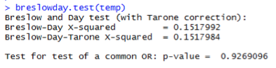
For the boy scout example, the Breslow-Day statistic is 0.15 with df = 2, p-value = 0.93. We do NOT have sufficient evidence to reject the model of homogeneous associations. Furthermore, the evidence is strong that associations are very similar across different levels of socioeconomic status.
The expected odds ratio for each table are: \(\hat{\theta}_{BD(high)}=1.20\approx \hat{\theta}_{BD(mild)}=0.89\approx \hat{\theta}_{BD(low)}=1.02\)
In this case, the common odds estimate from CMH test is a good estimate of the above values, i.e., common OR=0.978 with 95% confidence interval (0.597, 1.601).
Of course, this was to be expected for this example, since we already concluded that the conditional independence model fits well, and the conditional independence model is a special case of the homogeneous association model.
We will see more about these models and functions in both R and SAS in the upcoming lessons.
Example - Graduate Admissions
Next, let's see how this works for the Berkeley admissions data. Recall that we set \(X=\) sex, \(Y=\) admission status, and \(Z=\) department. The question of bias in admission can be approached with two tests characterized by the following null hypotheses: 1) sex is marginally independent of admission, and 2) sex and admission are conditionally independent, given department.
For the test of marginal independence of sex and admission, the Pearson test statistic is \(X^2 = 92.205\) with df = 1 and p-value approximately zero. All the expected values are greater than five, so we can rely on the large sample chi-square approximation to conclude that sex and admission are significantly related. More specifically, the estimated odds ratio, 0.5423, with 95% confidence interval (0.4785, 0.6147) indicates that the odds of acceptance for males are about two times as high as that for females.
What about this relationship viewed within a particular department? The CMH test statistic of 1.5246 with df = 1 and p-value = 0.2169 indicates that sex and admission are not (significantly) conditionally related, given department. The Mantel-Haenszel estimate of the common odds ratio is \(0.9047=1/1.1053\) with 95% CI \((0.7719, 1.0603)\). However, the Breslow-Day statistic testing for the homogeneity of the odds ratio is 18.83 with df = 5 and p-value = 0.002!
5.4 - Modeling Strategy
5.4 - Modeling StrategyWith three variables, there are nine possible models. The order here is from the most complex to simple.
| Saturated | (\(XYZ\)) |
|---|---|
| Homogeneous associations | \((XY, XZ, YZ)\) |
| Conditional independence (3 different models) | (\(XY, XZ\)) (\(XY, YZ\)) (\(XZ, YZ\)) |
| Joint independence (3 different models) | (\(XY, Z\)) (\(XZ, Y\)) (\(X, XZ\)) |
| Complete independence | (\(X, Y, Z\)) |
Any model that lies below a given model is a special case of the more complex model(s). Such structure among models is known as hierarchical model structure. With real data, we may not want to fit all of these models but focus only on those that make sense. For example, suppose that \(Z\) (e.g. admission) can be regarded as a response variable, and \(X\) (e.g., sex) and \(Y\) (e.g., department) are predictors.
- In regression, we do not model the relationships among predictors but allow arbitrary associations among them. Therefore, the simplest model that we may wish to fit is a null model \((XY, Z)\) which says that neither predictor is related to the response.
- If the null model does not fit, then we should try \((XY, XZ)\), which says that \(X\) is related to \(Z\), but \(Y\) is not. As we will see later in the course, this is equivalent to a logistic regression for \(Z\) with a main effect for \(X\) but no effect for \(Y\).
- We may also try \((XY, YZ)\), which is equivalent to a logistic regression for \(Z\) with a main effect for \(Y\) but no effect for \(X\).
- If neither of those models fit, we may try the model of homogeneous association, \((XY, YZ, XZ)\), which is equivalent to a logistic regression for \(Z\) with main effects for \(X\) and for \(Y\) but no interaction.
- The saturated model \((XYZ)\) is equivalent to a logistic regression for \(Z\) with a main effect for \(X\), a main effect for \(Y\), and an \(XY\) interaction.
We will learn more about model selection as we learn more about log-linear and logit models. As we consider more three-way and higher-way tables, models rather than single statistics or significance testing will give us a better sense of associations between variables and the nature of the dependencies.
Extensions to k-way tables are straightforward, and work by grouping. For example, consider six binary random variables: \(X_1,X_2,X_3,X_4,X_5\), and \(X_6\). These can be represented in a \(2^6\) table. The simplest model is the model of complete independence \(X_1,X_2,X_3,X_4,X_5,X_6\), and the saturated is the most complex one including all possible interactions. But now there are many more conditional and joint independence models that we can consider, but these can be reduced to three-way and two-way tables by grouping certain variables.
Let's say that now \(A=(X_1,X_2,)\), \(B=(X_3)\), and \(C=(X_4,X_5,X_6\)), and the joint independence model \((AB,C)\) says that \(X_1,X_2\), and \(X_3\) are jointly independent of \(X_4,X_5\), and \(X_6\). Basically, we can do the analysis of an \(AB \times C\), \(8\times 8\) table. We can also consider other joint and conditional independence models with other groupings of the variables. We will see more on model selection in the upcoming lessons.
5.5 - Lesson 5 Summary
5.5 - Lesson 5 SummaryIn this lesson, we explored the structure and potential associations between 3 categorical variables. We extended the concepts of testing for independence and associations from two-way to three-way tables. We introduced various types of associations, including marginal and conditional, and showed how the presence of a confounding variable can change or even reverse the relationship between the others.
Up to this point, we have been focusing on significance testing and summary measures of association. In what follows, we will switch gears and learn how to explain these associations by way of models and focus on estimating the parameters of the models. The advantage of the modeling approach is the additional flexibility to accommodate more variables and even quantitative predictors.