The Nearest Neighbor Classifier
Training data: \((g_i, x_i)\), \(i=1,2,\ldots,N\).
Problem: Over fitting
It is easy to overfit data. For example, assume we know that the data generating process has a linear boundary, but there is some random noise to our measurements.
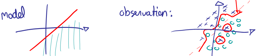
Solution: Smoothing
To prevent overfitting, we can smooth the decision boundary by K nearest neighbors instead of 1.
Find the K training samples \(x_r\), \(r = 1, \ldots , K\) closest in distance to \(x^*\), and then classify using majority vote among the k neighbors.
The amount of computation can be intense when the training data is large since the distance between a new data point and every training point has to be computed and sorted.
Feature standardization is often performed in pre-processing. Because standardization affects the distance, if one wants the features to play a similar role in determining the distance, standardization is recommended. However, whether to apply normalization is rather subjective. One has to decide on an individual basis for the problem in consideration.
The only parameter that can adjust the complexity of KNN is the number of neighbors k. The larger k is, the smoother the classification boundary. Or we can think of the complexity of KNN as lower when k increases.
The classification boundaries generated by a given training data set and 15 Nearest Neighbors are shown below. As a comparison, we also show the classification boundaries generated for the same training data but with 1 Nearest Neighbor. We can see that the classification boundaries induced by 1 NN are much more complicated than 15 NN.
15 Nearest Neighbors (below)
Figure 13.3 k-nearest-neighbor classifiers applied to the simulation data of figure 13.1. The broken purple curve in the background is the Bayes decision boundary.
1 Nearest Neighbor (below)
For another simulated data set, there are two classes. The error rates based on the training data, the test data, and 10 fold cross validation are plotted against K, the number of neighbors. We can see that the training error rate tends to grow when k grows, which is not the case for the error rate based on a separate test data set or cross-validation. The test error rate or cross-validation results indicate there is a balance between k and the error rate. When k first increases, the error rate decreases, and it increases again when k becomes too big. Hence, there is a preference for k in a certain range.
Figure 13.4 k-nearest-neighbors on the two-class mixture data. The upper panel shows the misclassification errors as a function of neighborhood size. Standard error bars are included for 10-fold cross validation. The lower panel shows the decision boundary for 7-nearest neighbors, which appears to be optimal for minimizing test error. The broken purple curve in the background is the Bayes decision boundary.
7 Nearest Neighbors (below)
Diabetes data
The diabetes data set is taken from the UCI machine learning database repository at: https://archive.ics.uci.edu/ml/datasets/Pima+Indians+Diabetes [1].
Load data into R as follows:
# set the working directory
setwd("C:/STAT 897D data mining")
# comma delimited data and no header for each variable
RawData <- read.table("diabetes.data",sep = ",",header=FALSE)
In RawData, the response variable is its last column; and the remaining columns are the predictor variables.
responseY <- as.matrix(RawData[,dim(RawData)[2]])
predictorX <- as.matrix(RawData[,1:(dim(RawData)[2]-1)])
For the convenience of visualization, we take the first two principle components as the new feature variables and conduct k-NN only on these two dimensional data.
pca <- princomp(predictorX, cor=T) # principal components analysis using correlation matrix
pc.comp <- pca$scores
pc.comp1 <- -1*pc.comp[,1]
pc.comp2 <- -1*pc.comp[,2]
In R, knn performs KNN and it is in the class library. Again, we take the first two PCA components as the predictor variables.
library(class)
X.train <- cbind(pc.comp1, pc.comp2)
model.knn <- knn(train=X.train, test=X.train, cl=responseY, k=19, prob=T)
In the above example, we set k = 19 due to the follow reason. To assess the classification accuracy, randomly split cross validation is used to compute the error rate. The samples are split into 20% for test dataset and 80% for training dataset. Fig. 1 shows the misclassification rates based on different k in KNN.
Figure 1: Training and test error rates based on cross-validation by K-NN with different k’s.
Based on Fig. 1, k = 19 yields the smallest test error rates. Therefore, we choose 19 as the best number of neighbors for KNN in this example. The classification result based on k = 19 is shown in the scatter plot of Fig. 2. The red circles represent Class 1, with diabetes, and the blue circles Class 0, non diabetes.
Figure 2: Classification result based on KNN with k = 19 for the Diabetes data.
The knn function also allows leave-one-out cross-validation, which in this case suggests k=17 is optimal. Results are very similar to those for k=19.
After completing the reading for this lesson, please finish the Quiz and R Lab on ANGEL (check the course schedule for due dates).
Links:
[1] https://archive.ics.uci.edu/ml/datasets/Pima+Indians+Diabetes