6.3 - Principal Components Analysis (PCA)

Objective

Capture the intrinsic variability in the data.

Reduce the dimensionality of a data set, either to ease interpretation or as a way to avoid overfitting and to prepare for subsequent analysis.

The sample covariance matrix of $\mathbf{X}$ is $\mathbf{S} = \mathbf{X}^T\mathbf{X}/\mathbf{N}$, since $\mathbf{X}$ has zero mean.

Eigen decomposition of $\mathbf{X}^T\mathbf{X}$:

$$\mathbf{X}^T\mathbf{X} = (\mathbf{U}\mathbf{D}\mathbf{V}^T)^T (\mathbf{U}\mathbf{D}\mathbf{V}^T) =\mathbf{V}\mathbf{D}^T\mathbf{U}^T\mathbf{U}\mathbf{D}\mathbf{V}^T = \mathbf{V}\mathbf{D}^2\mathbf{V}^T$$

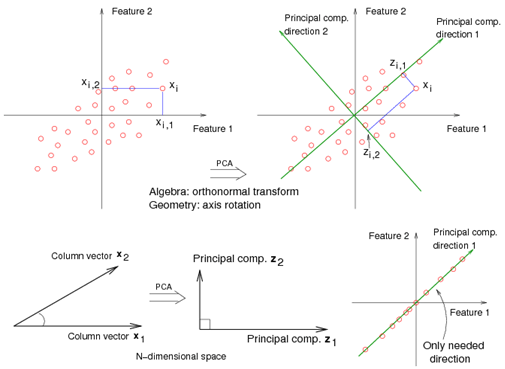
The eigenvectors of $\mathbf{X}^T\mathbf{X}$ (i.e., v_j, j = 1, …, p) are called principal component directions of $\mathbf{X}$.

The first principal component direction $\mathbf{v}_1$ has the following properties that

• $\mathbf{v}_1$ is the eigenvector associated with the largest eigenvalue, $\mathbf{d}_1^2$, of $\mathbf{X}^T\mathbf{X}$.
• $\mathbf{z}_1 = \mathbf{X}\mathbf{v}_1$ has the largest sample variance amongst all normalized linear combinations of the columns of X.
• $\mathbf{z}_1$ is called the first principal component of $\mathbf{X}$. And, we have $Var(\mathbf{z}_1)= d_1^2 / N$.

The second principal component direction v₂ (the direction orthogonal to the first component that has the largest projected variance) is the eigenvector corresponding to the second largest eigenvalue, $\mathbf{d}_2^2$ , of $\mathbf{X}^T\mathbf{X}$, and so on. (The eigenvector for the kth largest eigenvalue corresponds to the kth principal component direction $\mathbf{v}_k$.)

The kth principal component of $\mathbf{X}$, $\mathbf{z}_k$, has maximum variance $\mathbf{d}_1^2 / N$, subject to being orthogonal to the earlier ones.