Printer-friendly version

Objective

Capture the intrinsic variability in the data.

Reduce the dimensionality of a data set, either to ease interpretation or as a way to avoid overfitting and to prepare for subsequent analysis.

The sample covariance matrix of \(\mathbf{X}\) is \(\mathbf{S} = \mathbf{X}^T\mathbf{X}/\mathbf{N}\), since \(\mathbf{X}\) has zero mean.

Eigen decomposition of \(\mathbf{X}^T\mathbf{X}\):

\[\mathbf{X}^T\mathbf{X} = (\mathbf{U}\mathbf{D}\mathbf{V}^T)^T (\mathbf{U}\mathbf{D}\mathbf{V}^T) =\mathbf{V}\mathbf{D}^T\mathbf{U}^T\mathbf{U}\mathbf{D}\mathbf{V}^T = \mathbf{V}\mathbf{D}^2\mathbf{V}^T\]

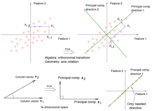
The eigenvectors of \(\mathbf{X}^T\mathbf{X}\) (i.e., v_j, j = 1, …, p) are called principal component directions of \(\mathbf{X}\).

The first principal component direction \(\mathbf{v}_1\) has the following properties that

• \(\mathbf{v}_1\) is the eigenvector associated with the largest eigenvalue, \(\mathbf{d}_1^2\), of \(\mathbf{X}^T\mathbf{X}\).
• \(\mathbf{z}_1 = \mathbf{X}\mathbf{v}_1\) has the largest sample variance amongst all normalized linear combinations of the columns of X.
• \(\mathbf{z}_1\) is called the first principal component of \(\mathbf{X}\). And, we have \(Var(\mathbf{z}_1)= d_1^2 / N\).

The second principal component direction v₂ (the direction orthogonal to the first component that has the largest projected variance) is the eigenvector corresponding to the second largest eigenvalue, \(\mathbf{d}_2^2\) , of \(\mathbf{X}^T\mathbf{X}\), and so on. (The eigenvector for the kth largest eigenvalue corresponds to the kth principal component direction \(\mathbf{v}_k\).)

The kth principal component of \(\mathbf{X}\), \(\mathbf{z}_k\), has maximum variance \(\mathbf{d}_1^2 / N\), subject to being orthogonal to the earlier ones.