In this section, we learn about the stepwise regression procedure. While we will soon learn the finer details, the general idea behind the stepwise regression procedure is that we build our regression model from a set of candidate predictor variables by entering and removing predictors — in a stepwise manner — into our model until there is no justifiable reason to enter or remove any more.

Our hope is, of course, that we end up with a reasonable and useful regression model. There is one sure way of ending up with a model that is certain to be underspecified — and that's if the set of candidate predictor variables doesn't include all of the variables that actually predict the response. This leads us to a fundamental rule of the stepwise regression procedure — the list of candidate predictor variables must include all of the variables that actually predict the response. Otherwise, we are sure to end up with a regression model that is underspecified and therefore misleading.

An example

Let's learn how the stepwise regression procedure works by considering a data set that concerns the hardening of cement. Sounds interesting, eh? In particular, the researchers were interested in learning how the composition of the cement affected the heat evolved during the hardening of the cement. Therefore, they measured and recorded the following data (cement.txt) on 13 batches of cement:

• Response y: heat evolved in calories during hardening of cement on a per gram basis
• Predictor x₁: % of tricalcium aluminate
• Predictor x₂: % of tricalcium silicate
• Predictor x₃: % of tetracalcium alumino ferrite
• Predictor x₄: % of dicalcium silicate

Now, if you study the scatter plot matrix of the data:

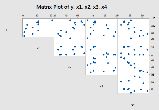
you can get a hunch of which predictors are good candidates for being the first to enter the stepwise model. It looks as if the strongest relationship exists between either y and x₂ or between y and x₄ — and therefore, perhaps either x₂ or x₄ should enter the stepwise model first. Did you notice what else is going on in this data set though? A strong correlation also exists between the predictors x₂ and x₄! How does this correlation among the predictor variables play out in the stepwise procedure? Let's see what happens when we use the stepwise regression method to find a model that is appropriate for these data.

Note. The number of predictors in this data set is not large. The stepwise procedure is typically used on much larger data sets, for which it is not feasible to attempt to fit all of the possible regression models. For the sake of illustration, the data set here is necessarily small, so that the largeness of the data set does not obscure the pedagogical point being made.

The procedure

Again, before we learn the finer details, let me again provide a broad overview of the steps involved. First, we start with no predictors in our "stepwise model." Then, at each step along the way we either enter or remove a predictor based on the partial F-tests — that is, the t-tests for the slope parameters — that are obtained. We stop when no more predictors can be justifiably entered or removed from our stepwise model, thereby leading us to a "final model."

Now, let's make this process a bit more concrete. Here goes:

Starting the procedure. The first thing we need to do is set a significance level for deciding when to enter a predictor into the stepwise model. We'll call this the Alpha-to-Enter significance level and will denote it as α_E. Of course, we also need to set a significance level for deciding when to remove a predictor from the stepwise model. We'll call this the Alpha-to-Remove significance level and will denote it as α_R. That is, first:

• Specify an Alpha-to-Enter significance level. This will typically be greater than the usual 0.05 level so that it is not too difficult to enter predictors into the model. Many software packages set this significance level by default to α_E = 0.15.
• Specify an Alpha-to-Remove significance level. This will typically be greater than the usual 0.05 level so that it is not too easy to remove predictors from the model. Again, many software packages set this significance level by default to α_R = 0.15.

Step #1. Once we've specified the starting significance levels, then we:

1. Fit each of the one-predictor models — that is, regress y on x₁, regress y on x₂, ..., and regress y on x_k.
2. Of those predictors whose t-test P-value is less than α_E = 0.15, the first predictor put in the stepwise model is the predictor that has the smallest t-test P-value.
3. If no predictor has a t-test P-value less than α_E = 0.15, stop.

Step #2. Then:

1. Suppose x₁ had the smallest t-test P-value below α_E = 0.15 and therefore was deemed the "best" single predictor arising from the the first step.
2. Now, fit each of the two-predictor models that include x₁ as a predictor — that is, regress y on x₁and x₂, regress y on x₁and x₃, ..., and regress y on x₁ and x_k.
3. Of those predictors whose t-test P-value is less than α_E = 0.15, the second predictor put in the stepwise model is the predictor that has the smallest t-test P-value.
4. If no predictor has a t-test P-value less than α_E = 0.15, stop. The model with the one predictor obtained from the first step is your final model.
5. But, suppose instead that x₂ was deemed the "best" second predictor and it is therefore entered into the stepwise model.
6. Now, since x₁ was the first predictor in the model, step back and see if entering x₂ into the stepwise model somehow affected the significance of the x₁ predictor. That is, check the t-test P-value for testing β₁ = 0. If the t-test P-value for β₁ = 0 has become not significant — that is, the P-value is greater than α_R = 0.15 — remove x₁ from the stepwise model.

Step #3. Then:

1. Suppose both x₁ and x₂ made it into the two-predictor stepwise model and remained there.
2. Now, fit each of the three-predictor models that include x₁ and x₂ as predictors — that is, regress y on x₁, x₂, and x₃, regress y on x₁, x₂, and x₄, ..., and regress y on x₁, x₂, and x_k.
3. Of those predictors whose t-test P-value is less than α_E = 0.15, the third predictor put in the stepwise model is the predictor that has the smallest t-test P-value.
4. If no predictor has a t-test P-value less than α_E = 0.15, stop. The model containing the two predictors obtained from the second step is your final model.
5. But, suppose instead that x₃ was deemed the "best" third predictor and it is therefore entered into the stepwise model.
6. Now, since x₁ and x₂ were the first predictors in the model, step back and see if entering x₃ into the stepwise model somehow affected the significance of the x₁ and x₂ predictors. That is, check the t-test P-values for testing β₁ = 0 and β₂ = 0. If the t-test P-value for either β₁ = 0 or β₂ = 0 has become not significant — that is, the P-value is greater than α_R = 0.15 — remove the predictor from the stepwise model.

Stopping the procedure. Continue the steps as described above until adding an additional predictor does not yield a t-test P-value below α_E = 0.15.

Whew! Let's return to our cement data example so we can try out the stepwise procedure as described above.

The example again

To start our stepwise regression procedure, let's set our Alpha-to-Enter significance level at α_E = 0.15, and let's set our Alpha-to-Remove significance level at α_R = 0.15. Now, regressing y on x₁, regressing y on x₂, regressing y on x₃, and regressing y on x₄, we obtain:

Each of the predictors is a candidate to be entered into the stepwise model because each t-test P-value is less than α_E = 0.15. The predictors x₂ and x₄ tie for having the smallest t-test P-value — it is 0.001 in each case. But note the tie is an artifact of rounding to three decimal places. The t-statistic for x₄ is larger in absolute value than the t-statistic for x₂—4.77 versus 4.69—and therefore the P-value for x₄ must be smaller. As a result of the first step, we enter x₄ into our stepwise model.

Now, following step #2, we fit each of the two-predictor models that include x₄ as a predictor — that is, we regress y on x₄ and x₁, regress y on x₄ and x₂, and regress y on x₄ and x₃, obtaining:

The predictor x₂ is not eligible for entry into the stepwise model because its t-test P-value (0.687) is greater than α_E = 0.15. The predictors x₁ and x₃ are candidates because each t-test P-value is less than α_E = 0.15. The predictors x₁ and x₃ tie for having the smallest t-test P-value—it is < 0.001 in each case. But, again the tie is an artifact of rounding to three decimal places. The t-statistic for x₁ is larger in absolute value than the t-statistic for x₃—10.40 versus 6.35—and therefore the P-value for x₁ must be smaller. As a result of the second step, we enter x₁ into our stepwise model.

Now, since x₄ was the first predictor in the model, we must step back and see if entering x₁ into the stepwise model affected the significance of the x₄ predictor. It did not—the t-test P-value for testing β₁ = 0 is less than 0.001, and thus smaller than α_R = 0.15. Therefore, we proceed to the third step with both x₁ and x₄ as predictors in our stepwise model.

Now, following step #3, we fit each of the three-predictor models that include x1 and x₄ as predictors — that is, we regress y on x₄, x₁, and x₂; and we regress y on x₄, x₁, and x₃, obtaining:

Both of the remaining predictors—x₂ and x₃—are candidates to be entered into the stepwise model because each t-test P-value is less than α_E = 0.15. The predictor x₂ has the smallest t-test P-value (0.052). Therefore, as a result of the third step, we enter x₂ into our stepwise model.

Now, since x₁ and x₄ were the first predictors in the model, we must step back and see if entering x₂ into the stepwise model affected the significance of the x₁ and x₄ predictors. Indeed, it did—the t-test P-value for testing β₄ = 0 is 0.205, which is greater than α_R = 0.15. Therefore, we remove the predictor x₄ from the stepwise model, leaving us with the predictors x₁ and x₂ in our stepwise model:

Now, we proceed fitting each of the three-predictor models that include x₁ and x₂ as predictors — that is, we regress y on x₁, x₂, and x₃; and we regress y on x₁, x₂, and x₄, obtaining:

Neither of the remaining predictors—x₃ and x₄—are eligible for entry into our stepwise model, because each t-test P-value—0.209 and 0.205, respectively—is greater than α_E = 0.15. That is, we stop our stepwise regression procedure. Our final regression model, based on the stepwise procedure contains only the predictors x₁ and x₂:

Whew! That took a lot of work! The good news is that most statistical software provides a stepwise regression procedure that does all of the dirty work for us.

Here's what stepwise regression output looks like for our cement data example:

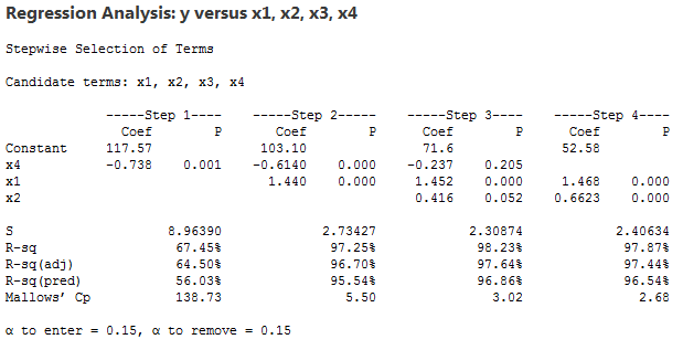
The output tells us that :

• a stepwise regression procedure was conducted on the response y and four predictors x₁, x₂, x₃, and x₄
• the Alpha-to-Enter significance level was set at α_E = 0.15 and the Alpha-to-Remove significance level was set at α_R = 0.15

The remaining portion of the output contains the results of the various steps of the stepwise regression procedure. One thing to keep in mind is that this output numbers the steps a little differently than described above. This output considers a step any addition or removal of a predictor from the stepwise model, whereas our steps—step #3, for example—considers the addition of one predictor and the removal of another as one step.

The results of each step are reported in a column labeled by the step number. It took four steps before the procedure was stopped. Here's what the output tells us:

• Just as our work above showed, as a result of the first step, the predictor x₄ is entered into the stepwise model. The output tells us that the estimated intercept ("Constant") b₀ = 117.57 and the estimated slope b₄ = -0.738. The P-value for testing β₄ = 0 is 0.001. The estimate S, which equals the square root of MSE, is 8.96. The R²-value is 67.45% and the adjusted R²-value is 64.50%. Mallows' Cp-statistic, which we learn about in the next section, is 138.73. The output also includes a predicted R²-value, which we'll come back to in Section 10.5.
• As a result of the second step, the predictor x₁ is entered into the stepwise model already containing the predictor x₄. The output tells us that the estimated intercept b₀ = 103.10, the estimated slope b₄ = -0.614, and the estimated slope b₁ = 1.44. The P-value for testing β₄ = 0 is < 0.001. The P-value for testing β₁ = 0 is < 0.001. The estimate S is 2.73. The R²-value is 97.25% and the adjusted R²-value is 96.70%. Mallows' Cp-statistic is 5.5.
• As a result of the third step, the predictor x₂ is entered into the stepwise model already containing the predictors x₁ and x₄. The output tells us that the estimated intercept b₀ = 71.6, the estimated slope b₄ = -0.237, the estimated slope b₁ = 1.452, and the estimated slope b₂ = 0.416. The P-value for testing β₄ = 0 is 0.205. The P-value for testing β₁ = 0 is < 0.001. The P-value for testing β₂ = 0 is 0.052. The estimate S is 2.31. The R²-value is 98.23% and the adjusted R²-value is 97.64%. Mallows' Cp-statistic is 3.02.
• As a result of the fourth and final step, the predictor x₄ is removed from the stepwise model containing the predictors x₁, x₂, and x₄, leaving us with the final model containing only the predictors x₁ and x₂. The output tells us that the estimated intercept b₀ = 52.58, the estimated slope b₁ = 1.468, and the estimated slope b₂ = 0.6623. The P-value for testing β₁ = 0 is < 0.001. The P-value for testing β₂ = 0 is < 0.001. The estimate S is 2.41. The R²-value is 97.87% and the adjusted R²-value is 97.44%. Mallows' Cp-statistic is 2.68.

Does the stepwise regression procedure lead us to the "best" model? No, not at all! Nothing occurs in the stepwise regression procedure to guarantee that we have found the optimal model. Case in point! Suppose we defined the best model to be the model with the largest adjusted R²-value. Then, here, we would prefer the model containing the three predictors x₁, x₂, and x₄, because its adjusted R²-value is 97.64%, which is higher than the adjusted R²-value of 97.44% for the final stepwise model containing just the two predictors x₁ and x₂.

Again, nothing occurs in the stepwise regression procedure to guarantee that we have found the optimal model. This, and other cautions of the stepwise regression procedure, are delineated in the next section.

Cautions!

Here are some things to keep in mind concerning the stepwise regression procedure:

• The final model is not guaranteed to be optimal in any specified sense.
• The procedure yields a single final model, although there are often several equally good models.
• Stepwise regression does not take into account a researcher's knowledge about the predictors. It may be necessary to force the procedure to include important predictors.
• One should not over-interpret the order in which predictors are entered into the model.
• One should not jump to the conclusion that all the important predictor variables for predicting y have been identified, or that all the unimportant predictor variables have been eliminated. It is, of course, possible that we may have committed a Type I or Type II error along the way.
• Many t-tests for testing β_k = 0 are conducted in a stepwise regression procedure. The probability is therefore high that we included some unimportant predictors or excluded some important predictors.

It's for all of these reasons that one should be careful not to overuse or overstate the results of any stepwise regression procedure.

More examples

Let's close up our discussion of stepwise regression by taking a quick look at two more examples.

Example #1. Are a person's brain size and body size predictive of his or her intelligence? Interested in this question, some researchers (Willerman, et al, 1991) collected the following data (iqsize.txt) on a sample of n = 38 college students:

• Response (y): Performance IQ scores (PIQ) from the revised Wechsler Adult Intelligence Scale. This variable served as the investigator's measure of the individual's intelligence.
• Potential predictor (x₁): Brain size based on the count obtained from MRI scans (given as count/10,000).
• Potential predictor (x₂): Height in inches.
• Potential predictor (x₃): Weight in pounds.

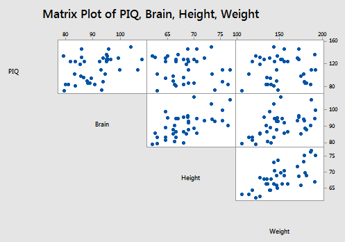
A matrix plot of the resulting data looks like:

Using statistical software to perform the stepwise regression procedure, we obtain:

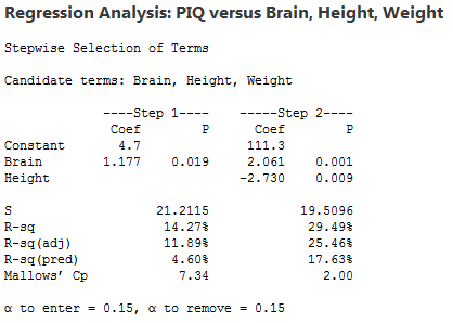
The output tells us:

• The first predictor entered into the stepwise model is Brain. The output tells us that the estimated intercept is 4.7 and the estimated slope for Brain is 1.177. The P-value for testing β_Brain = 0 is 0.019. The estimate S is 21.2, the R²-value is 14.27%, the adjusted R²-value is 11.89%, and Mallows' Cp-statistic is 7.34.
• The second and final predictor entered into the stepwise model is Height. The output tells us that the estimated intercept is 111.3, the estimated slope for Brain is 2.061, and the estimated slope for Height is -2.730. The P-value for testing β_Brain = 0 is 0.001. The P-value for testing β_Height = 0 is 0.009. The estimate S is 19.5, the R²-value is 29.49%, the adjusted R²-value is 25.46%, and Mallows' Cp-statistic is 2.00.
• At no step is a predictor removed from the stepwise model.
• When α_E = α_R = 0.15, the final stepwise regression model contains the predictors Brain and Height.

Example #2. Some researchers observed the following data (bloodpress.txt) on 20 individuals with high blood pressure:

• blood pressure (y = BP, in mm Hg)
• age (x₁ = Age, in years)
• weight (x₂ = Weight, in kg)
• body surface area (x₃ = BSA, in sq m)
• duration of hypertension (x₄ = Dur, in years)
• basal pulse (x₅ = Pulse, in beats per minute)
• stress index (x₆ = Stress)

The researchers were interested in determining if a relationship exists between blood pressure and age, weight, body surface area, duration, pulse rate and/or stress level.

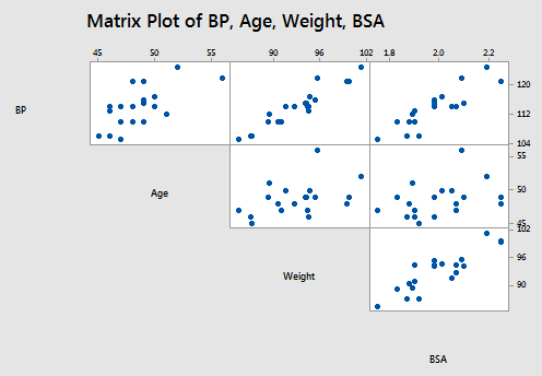
The matrix plot of BP, Age, Weight, and BSA looks like:

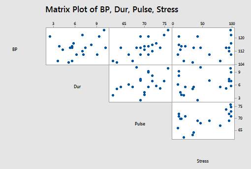
and the matrix plot of BP, Dur, Pulse, and Stress looks like:

Using statistical software to perform the stepwise regression procedure, we obtain:

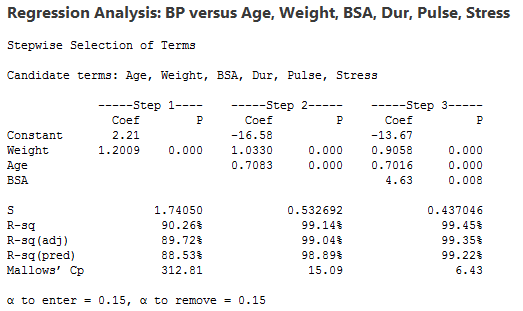
When α_E = α_R = 0.15, the final stepwise regression model contains the predictors Weight, Age, and BSA.