In this section, we learn about the best subsets regression procedure (or the all possible subsets regression procedure). While we will soon learn the finer details, the general idea behind best subsets regression is that we select the subset of predictors that do the best at meeting some well-defined objective criterion, such as having the largest R² value or the smallest MSE.

Again, our hope is that we end up with a reasonable and useful regression model. There is one sure way of ending up with a model that is certain to be underspecified—and that's if the set of candidate predictor variables doesn't include all of the variables that actually predict the response. Therefore, just as is the case for the stepwise regression procedure, a fundamental rule of the best subsets regression procedure is that the list of candidate predictor variables must include all of the variables that actually predict the response. Otherwise, we are sure to end up with a regression model that is underspecified and therefore misleading.

The procedure

A regression analysis utilizing the best subsets regression procedure involves the following steps:

Step #1. First, identify all of the possible regression models derived from all of the possible combinations of the candidate predictors. Unfortunately, this can be a huge number of possible models.

For the sake of example, suppose we have k=3 candidate predictors—x₁, x₂, and x₃—for our final regression model. Then, there are 2³=8 possible regression models we can consider:

• the one (1) model with no predictors
• the three (3) models with only one predictor each — the model with x₁ alone; the model with x₂ alone; and the model with x₃ alone
• the three (3) models with two predictors each — the model with x₁ and x₂; the model with x₁ and x₃; and the model with x₂ and x₃
• and the one (1) model with all three predictors — that is, the model with x₁, x₂ and x₃

That's 1 + 3 + 3 + 1 = 8 possible models to consider. It can be shown that when there are four candidate predictors—x₁, x₂, x₃ and x₄—there are 16 possible regression models to consider. In general, if there are k possible candidate predictors, then there are 2^k possible regression models containing the predictors. For example, 10 predictors yield 2¹⁰ = 1024 possible regression models.

That's a heck of a lot of models to consider! The good news is that statistical software does all of the dirty work for us.

Step #2. From the possible models identified in the first step, determine the one-predictor models that do the "best" at meeting some well-defined criteria, the two-predictor models that do the "best," the three-predictor models that do the "best," and so on. For example, suppose we have three candidate predictors—x₁, x₂, and x₃—for our final regression model. Of the three possible models with one predictor, identify the one or two that does "best." Of the three possible two-predictor models, identify the one or two that does "best." By doing this, it cuts down considerably the number of possible regression models to consider!

But, have you noticed that we have not yet even defined what we mean by "best"? What do you think "best" means? Of course, you'll probably define it differently than me or than your neighbor. Therein lies the rub—we might not be able to agree on what's best! In thinking about what "best" means, you might have thought of any of the following:

• the model with the largest R²
• the model with the largest adjusted R²
• the model with the smallest MSE (or S = square root of MSE)

There are other criteria you probably didn't think of, but we could consider, too, for example, Mallows' C_p-statistic, the PRESS statistic, and Predicted R² (which is calculated from the PRESS statistic). We'll learn about Mallows' C_p-statistic in this section and about the PRESS statistic and Predicted R² in Section 11.5.

To make matters even worse—the different criteria quantify different aspects of the regression model, and therefore often yield different choices for the best set of predictors. That's okay—as long as we don't misuse best subsets regression by claiming that it yields the best model. Rather, we should use best subsets regression as a screening tool—that is, as a way to reduce the large number of possible regression models to just a handful of models that we can evaluate further before arriving at one final model.

Step #3. Further evaluate and refine the handful of models identified in the last step. This might entail performing residual analyses, transforming the predictors and/or response, adding interaction terms, and so on. Do this until you are satisfied that you have found a model that meets the model conditions, does a good job of summarizing the trend in the data, and most importantly allows you to answer your research question.

An example

For the remainder of this section, we discuss how the criteria identified above can help us reduce the large number of possible regression models to just a handful of models suitable for further evaluation.

For the sake of example, we will use the cement data to illustrate use of the criteria. Therefore, let's quickly review—the researchers measured and recorded the following data (cement.txt) on 13 batches of cement:

• Response y: heat evolved in calories during hardening of cement on a per gram basis
• Predictor x₁: % of tricalcium aluminate
• Predictor x₂: % of tricalcium silicate
• Predictor x₃: % of tetracalcium alumino ferrite
• Predictor x₄: % of dicalcium silicate

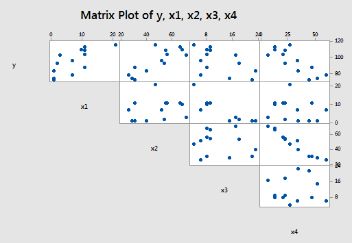
And, the matrix plot of the data looks like:

The R²-values

As you may recall, the R²-value, which is defined as:

\[R^2=\frac{SSR}{SSTO}=1-\frac{SSE}{SSTO}\]

can only increase as more variables are added. Therefore, it makes no sense to define the "best" model as the model with the largest R²-value. After all, if we did, the model with the largest number of predictors would always win.

All is not lost, however. We can instead use the R²-values to find the point where adding more predictors is not worthwhile, because it yields a very small increase in the R²-value. In other words, we look at the size of the increase in R², not just its magnitude alone. Because this is such a "wishy-washy" criteria, it is used most often in combination with the other criteria.

Let's see how this criterion works on the cement data example.

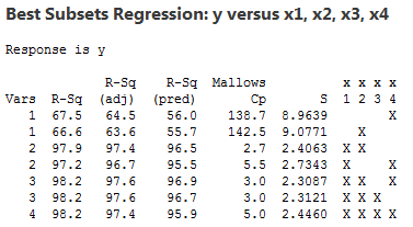
Each row in the table represents information about one of the possible regression models. The first column—labeled Vars—tells us how many predictors are in the model. The last four columns—labeled downward x1, x2, x3, and x4—tell us which predictors are in the model. If an "X" is present in the column, then that predictor is in the model. Otherwise, it is not. For example, the first row in the table contains information about the model in which x₄ is the only predictor, whereas the fourth row contains information about the model in which x₁ and x₄ are the two predictors in the model. The other five columns—labeled R-sq, R-sq(adj), R-sq(pred), Cp and S—pertain to the criteria that we use in deciding which models are "best."

As you can see, this output reports only the two best models for each number of predictors based on the size of the R²-value—that is, the output reports the two one-predictor models with the largest R²-values, followed by the two two-predictor models with the largest R²-values, and so on.

So, using the R²-value criterion, which model (or models) should we consider for further evaluation? Hmmm—going from the "best" one-predictor model to the "best" two-predictor model, the R²-value jumps from 67.5 to 97.9. That is a jump worth making! That is, with such a substantial increase in the R²-value, one could probably not justify—with a straight face at least—using the one-predictor model over the two-predictor model. Now, should we instead consider the "best" three-predictor model? Probably not! The increase in the R²-value is very small—from 97.9 to 98.2—and therefore, we probably can't justify using the larger three-predictor model over the simpler, smaller two-predictor model. Get it? Based on the R²-value criterion, the "best" model is the model with the two predictors x₁ and x₂.

The adjusted R²-value and MSE

The adjusted R²-value, which is defined as:

\[R_{a}^{2}=1-\left(\frac{n-1}{n-k-1}\right)\left(\frac{SSE}{SSTO}\right)=1-\left(\frac{n-1}{SSTO}\right)MSE=\frac{\frac{SSTO}{n-1}-\frac{SSE}{n-k-1}}{\frac{SSTO}{n-1}}\]

makes us pay a penalty for adding more predictors to the model. Therefore, we can just use the adjusted R²-value outright. That is, according to the adjusted R²-value criterion, the best regression model is the one with the largest adjusted R²-value.

Now, you might have noticed that the adjusted R²-value is a function of the mean square error (MSE). And, you may—or may not—recall that MSE is defined as:

\[MSE=\frac{SSE}{n-k-1}=\frac{\sum(y_i-\hat{y}_i)^2}{n-k-1}\]

That is, MSE quantifies how far away our predicted responses are from our observed responses. Naturally, we want this distance to be small. Therefore, according to the MSE criterion, the best regression model is the one with the smallest MSE.

But, aha—the two criteria are equivalent! If you look at the formula again for the adjusted R²-value:

\[R_{a}^{2}=1-\left(\frac{n-1}{SSTO}\right)MSE\]

you can see that the adjusted R²-value increases only if MSE decreases. That is, the adjusted R²-value and MSE criteria always yield the same "best" models.

Back to the cement data example! One thing to note is that S is the square root of MSE. Therefore, finding the model with the smallest MSE is equivalent to finding the model with the smallest S:

The model with the largest adjusted R²-value (97.6) and the smallest S (2.3087) is the model with the three predictors x₁, x₂, and x₄.

See?! Different criteria can indeed lead us to different "best" models. Based on the R²-value criterion, the "best" model is the model with the two predictors x₁ and x₂. But, based on the adjusted R²-value and the smallest MSE criteria, the "best" model is the model with the three predictors x₁, x₂, and x₄.

Mallows' C_p-statistic

Recall that an underspecified model is a model in which important predictors are missing. And, an underspecified model yields biased regression coefficients and biased predictions of the response. Well, in short, Mallows' C_p-statistic estimates the size of the bias that is introduced into the predicted responses by having an underspecified model.

Now, we could just jump right in and be told how to use Mallows' C_p-statistic as a way of choosing a "best" model. But, then it wouldn't make any sense to you—and therefore it wouldn't stick to your craw. So, we'll start by justifying the use of the Mallows' C_p-statistic. The problem is it's kind of complicated. So, be patient, don't be frightened by the scary looking formulas, and before you know it, we'll get to the moral of the story. Oh, and by the way, in case you're wondering—it's called Mallows' C_p-statistic, because a guy named Mallows thought of it!

Here goes! At issue in any regression model are two things, namely:

• The bias in the predicted responses.
• The variation in the predicted responses.

Bias in predicted responses

Recall that, in fitting a regression model to data, we attempt to estimate the average—or expected value—of the observed responses E(y_i) at any given predictor value x. That is, E(y_i) is the population regression function. Because the average of the observed responses depends on the value of x, we might also denote this population average or population regression function as μ_Y|x.

Now, if there is no bias in the predicted responses, then the average of the observed responses E(y_i) and the average of the predicted responses E(\(\hat{y}_i\)) both equal the thing we are trying to estimate, namely the average of the responses in the population μ_Y|x. On the other hand, if there is bias in the predicted responses, then E(y_i) = μ_Y|x and E(\(\hat{y}_i\)) do not equal each other. The difference between E(y_i) and E(\(\hat{y}_i\)) is the bias B_i in the predicted response. That is, the bias:

\[B_i=E(\hat{y}_i)-E(y_i)\]

We can picture this bias as follows:

The quantity E(y_i) is the value of the population regression line at a given x. Recall that we assume that the error terms ε_i are normally distributed. That's why there is a normal curve—in blue—drawn around the population regression line E(y_i). You can think of the quantity E(\(\hat{y}_i\)) as being the predicted regression line—well, technically, it's the average of all of the predicted regression lines you could obtain based on your formulated regression model. Again, since we always assume the error terms ε_i are normally distributed, we've drawn a normal curve—in red—around the average predicted regression line E(\(\hat{y}_i\)). The difference between the population regression line E(y_i) and the average predicted regression line E(\(\hat{y}_i\)) is the bias \(B_i=E(\hat{y}_i)-E(y_i)\) .

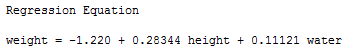
Earlier in this lesson, we saw an example in which bias was likely introduced into the predicted responses because of an underspecifed model. The data concerned the heights and weights of martians. The data set (martian.txt) contains the weights (in g), heights (in cm), and amount of daily water consumption (0, 10 or 20 cups per day) of 12 martians.

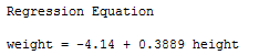
If we regress y = weight on the predictors x₁ = height and x₂ = water, we obtain the following estimated regression equation:

But, if we regress y = weight on only the one predictor x₁ = height, we obtain the following estimated regression equation:

A plot of the data containing the two estimated regression equations looks like:

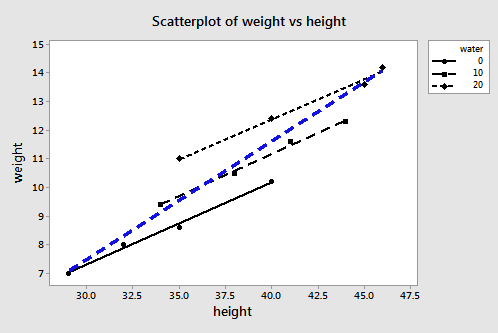
The three black lines represent the estimated regression equation when the amount of water consumption is taken into account — the first line for 0 cups per day, the second line for 10 cups per day, and the third line for 20 cups per day. The dashed blue line represents the estimated regression equation when we leave the amount of water consumed out of the regression model.

As you can see, if we use the blue line to predict the weight of a randomly selected martian, we would consistently overestimate the weight of martians who drink 0 cups of water a day, and we would consistently understimate the weight of martians who drink 20 cups of water a day. That is, our predicted responses would be biased.

Variation in predicted responses

When a bias exists in the predicted responses, the variance in the predicted responses for a data point i is due to two things:

• the ever-present random sampling variation, that is \((\sigma_{\hat{y}_i}^{2})\)
• the variance associated with the bias, that is \((B_{i}^{2})\)

Now, if our regression model is biased, it doesn't make sense to consider the bias at just one data point i. We need to consider the bias that exists for all n data points. Looking at the plot of the two estimated regression equations for the martian data, we see that the predictions for the underspecified model are more biased for certain data points than for others. And, we can't just consider the variation in the predicted responses at one data point i. We need to consider the total variation in the predicted responses.

To quantify the total variation in the predicted responses, we just sum the two variance components—\((\sigma_{\hat{y}_i}^{2})\) and \((B_{i}^{2})\)—over all n data points to obtain a (standardized) measure of the total variation in the predicted responses Γ_p (that's the greek letter "gamma"):

\[\Gamma_p=\frac{1}{\sigma^2} \left\{ \sum_{i=1}^{n}\sigma_{\hat{y}_i}^{2}+\sum_{i=1}^{n}\left[ E(\hat{y}_i)-E(y_i) \right] ^2 \right\}\]

I warned you about not being overwhelmed by scary looking formulas! The first term in the brackets quantifies the random sampling variation summed over all n data points, while the second term in the brackets quantifies the amount of bias (squared) summed over all n data points. Because the size of the bias depends on the measurement units used, we divide by σ² to get a standardized unitless measure.

Now, we don't have the tools to prove it, but it can be shown that if there is no bias in the predicted responses—that is, if the bias = 0—then Γ_p achieves its smallest possible value, namely k+1, the number of parameters:

\[\Gamma_p=\frac{1}{\sigma^2} \left\{ \sum_{i=1}^{n}\sigma_{\hat{y}_i}^{2}+0 \right\}=k+1\]

Now, because it quantifies the amount of bias and variance in the predicted responses, Γ_p seems to be a good measure of an underspecified model:

\[\Gamma_p=\frac{1}{\sigma^2} \left\{ \sum_{i=1}^{n}\sigma_{\hat{y}_i}^{2}+\sum_{i=1}^{n} \left[ E(\hat{y}_i)-E(y_i) \right] ^2 \right\}\]

The best model is simply the model with the smallest value of Γ_p. We even know that the theoretical minimum of Γ_p is the number of parameters k+1.

Well, it's not quite that simple—we still have a problem. Did you notice all of those greek parameters—σ², \((\sigma_{\hat{y}_i}^{2})\), and Γ_p? As you know, greek parameters are generally used to denote unknown population quantities. That is, we don't or can't know the value of Γ_p—we must estimate it. That's where Mallows' C_p-statistic comes into play!

C_p as an estimate of Γ_p

If we know the population variance σ², we can estimate Γ_p:

\[C_p=k+1+\frac{(MSE_k-\sigma^2)(n-k-1)}{\sigma^2}\]

where MSE_k is the mean squared error from fitting the model containing the subset of k predictors.

But we don't know σ². So, we estimate it using MSE_all, the mean squared error obtained from fitting the model containing all of the candidate predictors. That is:

\[C_p=k+1+\frac{(MSE_k-MSE_{all})(n-k-1)}{MSE_{all}}=k+1+\frac{(n-k-1)MSE_k}{MSE_{all}}-(n-k-1)=\frac{SSE_k}{MSE_{all}}+2(k+1)-n.\]

A couple of things to note though. Estimating σ² using MSE_all:

• assumes that there are no biases in the full model with all of the predictors, an assumption that may or may not be valid, but can't be tested without additional information (at the very least you have to have all of the important predictors involved)
• guarantees that C_p = k+1 for the full model because in that case MSE_k = MSE_all.

Using the C_p criterion to identify "best" models

Finally—we're getting to the moral of the story! Just a few final facts about Mallows' C_p-statistic will get us on our way. Recalling that k denotes the number of predictor terms in the model:

• Subset models with small C_p values have a small estimated total (standardized) variation in predicted responses.
• When the C_p value is ...
  • ... near k+1, the bias is small (next to none)
  • ... much greater than k+1, the bias is substantial
  • ... below k+1, it is due to sampling error; interpret as no bias
• For the largest model containing all of the candidate predictors, C_p = k+1 (always). Therefore, you shouldn't use C_p to evaluate the full model (the model containing all of the candiate predictors).

That all said, here's a reasonable strategy for using C_p to identify "best" models:

• Identify subsets of predictors for which the C_p value is near k+1 (if possible).
• The full model always yields C_p = k+1, so don't select the full model based on C_p.
• If all models, except the full model, yield a large C_p not near k+1, it suggests some important predictor(s) are missing from the analysis. In this case, we are well-advised to identify the predictors that are missing!
• If a number of models have C_p near k+1, choose the model with the smallest C_p value, thereby insuring that the combination of the bias and the variance is at a minimum.
• When more than one model has a small value of C_p value near k+1, in general, choose the simpler model or the model that meets your research needs.

The cement data example

Ahhh—an example! Let's see what model the C_p criterion leads us to for the cement data:

The first thing you might want to do here is "pencil in" a column to the left of the Vars column. Recall that the Vars column tells us the number of predictor terms (k) that are in the model. But, we need to compare C_p to the number of parameters (k+1). There is always one more parameter—the intercept parameter—than predictor terms. So, you might want to add—at least mentally—a column containing the number of parameters—here, 2, 2, 3, 3, 4, 4, and 5.

Here, the model in the third row (containing predictors x₁ and x₂), the model in the fifth row (containing predictors x₁, x₂ and x₄), and the model in the sixth row (containing predictors x₁, x₂ and x₃) are all unbiased models, because their C_p values equal (or are below) the number of parameters k+1. For example:

• the model containing the predictors x₁ and x₂ contains 3 parameters and its C_p value is 2.7. Since C_p is less than k+1=3, it suggests the model is unbiased;
• the model containing the predictors x₁, x₂ and x₄ contains 4 parameters and its C_p value is 3.0. Since C_p is less than k+1=4, it suggests the model is unbiased;
• the model containing the predictors x₁, x₂ and x₃ contains 4 parameters and its C_p value is 3.0. Since C_p is less than k+1=4, it suggests the model is unbiased.

So, in this case, based on the C_p criterion, the researcher has three legitimate models from which to choose with respect to bias. Of these three, the model containing the predictors x₁ and x₂ has the smallest C_p value, but the C_p values for the other two models are similar and so there is little to separate these models based on this criterion.

Incidentally, you might also want to conclude that the last model—the model containing all four predictors—is a legitimate contender because C_p = 5.0 equals k+1 = 5. However, don't forget that the model with all of the predictor terms is assumed to be unbiased. Therefore, you should not use the C_p criterion as a way of evaluating the full model with all of the candidate predictor terms.

Incidentally, how did the statistical software detemine that the C_p value for the third model is 2.7, while for the fourth model the C_p value is 5.5? We can verify these calculated C_p values!

First, consider the third model containing the predictors x₁ and x₂ for which k=2. The following output obtained by first regressing y on the predictors x₁, x₂, x₃ and x₄ and then by regressing y on the predictors x₁ and x₂ :

tells us that, here, SSE_k = 57.9 and MSE_all = 5.98 . Therefore, just as the output claims:

\[C_p= \frac{SSE_k}{MSE_{all}}+2(k+1)-n = \frac{57.9}{5.98}+2(2+1)-13=2.7. \]

Next, consider the fourth model containing the predictors x₁ and x₄ for which k =2. The following output obtained by first regressing y on the predictors x₁, x₂, x₃ and x₄ and then by regressing y on the predictors x₁ and x₄:

tells us that, here, SSE_k = 74.8 and MSE_all = 5.98 . Therefore, just as the output claims:

\[C_p= \frac{SSE_k}{MSE_{all}}+2(k+1)-n = \frac{74.8}{5.98}+2(2+1)-13=5.5. \]