11.6 - Further Automated Variable Selection Examples
Example: Peruvian Blood Pressure Data
 First we will illustrate the “Best Subsets” procedure and a “by hand” calculation of the information criteria from earlier. Recall from Lesson 5 that this dataset consists of variables possibly relating to blood pressures of n = 39 Peruvians who have moved from rural high altitude areas to urban lower altitude areas (peru.txt). The variables in this dataset (where we have omitted the calf skinfold variable from the first time we used this example) are:
Y = systolic blood pressure
X1 = age
X2 = years in urban area
X3 = X2 /X1 = fraction of life in urban area
X4 = weight (kg)
X5 = height (mm)
X6 = chin skinfold
X7 = forearm skinfold
X8 = resting pulse rate
The results from the best subsets procedure are presented below.
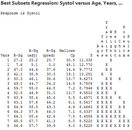
To interpret the results, we start by noting that the lowest Cp value (= 5.5) occurs for the five-variable model that includes the variables Age, Years, fraclife, Weight, and Chin. The ”X”s to the right side of the display tell us which variables are in the model (look up to the column heading to see the variable name). The value of R2 for this model is 63.9% and the value of R2adj is 58.4%. If we look at the best six-variable model, we see only minimal changes in these values, and the value of \(S = \sqrt{MSE}\) increases. A five-variable model most likely will be sufficient. We should then use multiple regression to explore the five-variable model just identified. Note that two of these x-variables relate to how long the person has lived at the urban lower altitude.
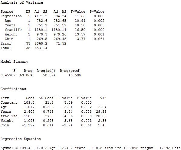
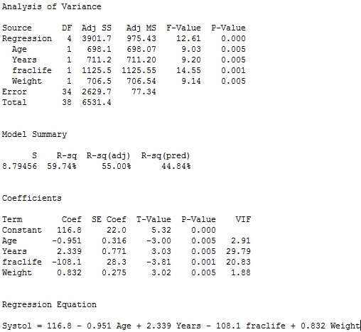
Next, we turn our attention to calculating AIC and BIC. Here are the multiple regression results for the best five-variable model (which has Cp = 5.5) and the best four-variable model (which has Cp = 7.2).
Best 5-variable model results:
Best 4-variable model results
AIC Comparison: The five-variable model still has a slight edge (a lower AIC is better).
- For the five-variable model:
AICk = 39 ln(2360.23) − 39 ln(39) + 2(6) = 172.015.
- For the four-variable model:
AICk = 39 ln(2629.71) − 39 ln(39) + 2(5) = 174.232.
BIC Comparison: The values are nearly the same; the five-variable model has a slightly lower value (a lower BIC is better).
- For the five-variable model:
BICk = 39 ln(2360.23) − 39 ln(39) + ln(39) × 6 = 181.997.
- For the four-variable model:
BICk = 39 ln(2629.71) − 39 ln(39) + ln(39) × 5 = 182.549.
Our decision is that the five-variable model has better values than the four-variable models, so it seems to be the winner. Interestingly, the Chin variable is not quite at the 0.05 level for significance in the five-variable model so we could consider dropping it as a predictor. But, the cost will be an increase in MSE and 4.2% drop in R2. Given the closeness of the Chin-value (0.061) to the 0.05 significance level and the relatively small sample size (39), we probably should keep the Chin variable in the model for prediction purposes. When we have a p-value that is only slightly higher than our significance level (by slightly higher, we mean usually no more than 0.05 above the significance level we are using), we usually say a variable is marginally significant. It is usually a good idea to keep such variables in the model, but one way or the other, you should state why you decided to keep or drop the variable.
Example: Measurements of College Students
 Next we will illustrate stepwise procedures. Recall from Lesson 5 that this dataset consists of n = 55 college students with measurements for the following seven variables (Physical.txt):
Y = height (in)
X1 = left forearm length (cm)
X2 = left foot length (cm)
X3 = left palm width
X4 = head circumference (cm)
X5 = nose length (cm)
X6 = gender, coded as 0 for male and 1 for female
Here is the output for a stepwise procedure.
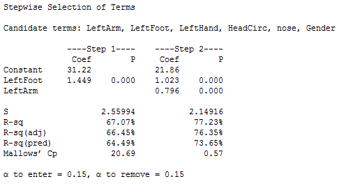
All six x-variables were candidates for the final model. The procedure took two forward steps and then stopped. The variables in the model at that point are left foot length and left forearm length. The left foot length variable was selected first (in Step 1), and then left forearm length was added to the model. The procedure stopped because no other variables could enter at a significant level. Notice that the significance level used for entering variables was 0.15. Thus, after Step 2 there were no more x-variables for which the p-value would be less than 0.15.
It is also possible to work backwards from a model with all the predictors included and only consider steps in which the least significant predictor is removed. Output for this backward elimination procedure is given below.
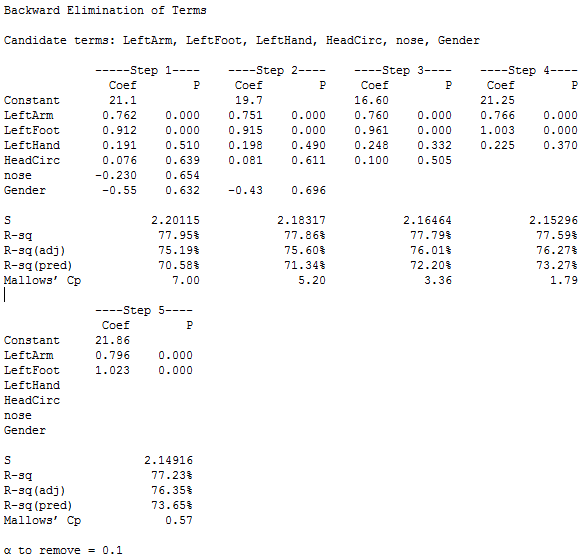
The procedure took five steps (counting Step 1 as the estimation of a model with all variables included). At each subsequent step, the weakest variable is eliminated until all variables in the model are significant (at the default 0.10 level). At a particular step, you can see which variable was eliminated by the new blank spot in the display (compared to the previous step). For instance, from Step 1 to Step 2, the nose length variable was dropped (it had the highest p-value.) Then, from Step 2 to Step 3, the gender variable was dropped, and so on.
The stopping point for the backward elimination procedure gave the same model as the stepwise procedure did, with left forearm length and left foot length as the only two x-variables in the model. It will not always necessarily be the case that the two methods used here will arrive at the same model.
Finally, it is also possible to work forwards from a base model with no predictors included and only consider steps in which the most significant predictor is added. We leave it as exercise to see how this forward selection procedure works for this dataset (you can probably guess given the results of the Stepwise procedure above).

