1.6 - Hypothesis Testing
Another way to make statistical inferences about a population parameter such as the mean is to use hypothesis testing to make decisions about the parameter’s value. Suppose that we are interested in a particular value of the mean single-family home sale price, for example, a claim from a realtor that the mean sale price in this market is \(\$\)255,000. Does the information in our sample support this claim, or does it favor an alternative claim?
The rejection region method
To decide between two competing claims, we can conduct a hypothesis test as follows.
- Express the claim about a specific value for the population parameter of interest as a null hypothesis, denoted NH. [More traditional notation uses H0.] The null hypothesis needs to be in the form "parameter = some hypothesized value," for example, NH: E(Y) = 255. A frequently used legal analogy is that the null hypothesis is equivalent to a presumption of innocence in a trial before any evidence has been presented.
- Express the alternative claim as an alternative hypothesis, denoted AH. [More traditional notation uses Ha or H1.]. The alternative hypothesis can be in a lower-tail form, for example, AH: E(Y) < 255, or an upper-tail form, for example, AH: E(Y) > 255, or a two-tail form, for example, AH: E(Y) ≠ 255. The alternative hypothesis, also sometimes called the research hypothesis, is what we would like to demonstrate to be the case, and needs to be stated before looking at the data. To continue the legal analogy, the alternative hypothesis is guilt, and we will only reject the null hypothesis (innocence) if we favor the alternative hypothesis (guilt) beyond a reasonable doubt. To illustrate, we will presume for the home prices example that we have some reason to suspect that the mean sale price is higher than claimed by the realtor (perhaps a political organization is campaigning on the issue of high housing costs and has employed us to investigate whether sale prices are "too high" in this housing market). Thus, our upper-tail alternative hypothesis is AH: E(Y) > 255.
- Calculate a test statistic based on the assumption that the null hypothesis is true. For hypothesis tests for a univariate population mean the relevant test statistic is \[\text{t-statistic}=\frac{m_Y-\text{E}(Y)}{s_Y/\sqrt{n}},\] where \(m_Y\) is the sample mean, E(Y) is the value of the population mean in the null hypothesis, \(s_Y\) is the sample standard deviation, and n is the sample size.
- Under the assumption that the null hypothesis is true, this test statistic will have a particular probability distribution. For testing a univariate population mean, this t-statistic has a t-distribution with n−1 degrees of freedom. We would therefore expect it to be "close" to zero (if the null hypothesis is true). Conversely, if it is far from zero, then we might begin to doubt the null hypothesis:
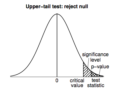
- For an upper-tail test, a t-statistic that is positive and far from zero would then lead us to favor the alternative hypothesis (a t-statistic that was far from zero but negative would favor neither hypothesis and the test would be inconclusive).
- For a lower-tail test, a t-statistic that is negative and far from zero would then lead us to favor the alternative hypothesis (a t-statistic that was far from zero but positive would favor neither hypothesis and the test would be inconclusive).
- For a two-tail test, any t-statistic that is far from zero (positive or negative) would lead us to favor the alternative hypothesis.
- To decide how far from zero a t-statistic would have to be before we reject the null hypothesis in favor of the alternative, recall the legal analogy. To deliver a guilty verdict (the alternative hypothesis), the jury must establish guilt beyond a reasonable doubt. In other words, a jury rejects the presumption of innocence (the null hypothesis) only if there is compelling evidence of guilt. In statistical terms, compelling evidence of guilt is found only in the tails of the t-distribution density curve. For example, in conducting an upper-tail test, if the t-statistic is way out in the upper tail, then it seems unlikely that the null hypothesis could have been true—so we reject it in favor of the alternative. Otherwise, the t-statistic could well have arisen while the null hypothesis held true—so we do not reject it in favor of the alternative. How far out in the tail does the t-statistic have to be to favor the alternative hypothesis rather than the null? Here we must make a decision about how much evidence we will require before rejecting a null hypothesis. There is always a chance that we might mistakenly reject a null hypothesis when it is actually true (the equivalent of pronouncing an innocent defendant guilty). Often, this chance—called the significance level—will be set at 5%, but more stringent tests (such as in clinical trials of new pharmaceutical drugs) might set this at 1%, while less stringent tests (such as in sociological studies) might set this at 10%. For the sake of argument, we use 5% as a default value for hypothesis tests in this course (unless stated otherwise).
- The significance level dictates the critical value(s) for the test, beyond which an observed t-statistic leads to rejection of the null hypothesis in favor of the alternative. This region, which leads to rejection of the null hypothesis, is called the rejection region. For example, for a significance level of 5%:
- For an upper-tail test, the critical value is the 95th percentile of the t-distribution with n−1 degrees of freedom; reject the null in favor of the alternative if the t-statistic is greater than this.
- For a lower-tail test, the critical value is the 5th percentile of the t-distribution with n−1 degrees of freedom; reject the null in favor of the alternative if the t-statistic is less than this.
- For a two-tail test, the two critical values are the 2.5th and the 97.5th percentiles of the t-distribution with n−1 degrees of freedom; reject the null in favor of the alternative if the t-statistic is less than the 2.5th percentile or greater than the 97.5th percentile.
It is best to lay out hypothesis tests in a series of steps, so for the house prices example:
- State null hypothesis: NH: E(Y) = 255.
- State alternative hypothesis: AH: E(Y) > 255.
- Calculate test statistic: t-statistic = \(m_Y−\text{E}(Y)/(s_Y/\sqrt{n})=(278.6033−255)/(53.8656/\sqrt{30})=2.40\).
- Set significance level: 5%.
- Look up critical value: The 95th percentile of the t-distribution with 29 degrees of freedom is 1.699; the rejection region is therefore any t-statistic greater than 1.699.
- Make decision: Since the t-statistic of 2.40 falls in the rejection region, we reject the null hypothesis in favor of the alternative.
- Interpret in the context of the situation: The 30 sample sale prices suggest that a population mean of \(\$\)255,000 seems implausible—the sample data favor a value greater than this (at a significance level of 5%).
The p-value method
An alternative way to conduct a hypothesis test is to again assume initially that the null hypothesis is true, but then to calculate the probability of observing a t-statistic as extreme as the one observed or even more extreme (in the direction that favors the alternative hypothesis). This is known as the p-value (sometimes also called the observed significance level):
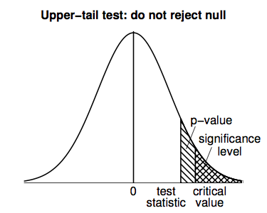
- For an upper-tail test, the p-value is the area under the curve of the t-distribution (with n−1 degrees of freedom) to the right of the observed t-statistic.
- For a lower-tail test, the p-value is the area under the curve of the t-distribution (with n−1 degrees of freedom) to the left of the observed t-statistic.
- For a two-tail test, the p-value is the sum of the areas under the curve of the t-distribution (with n−1 degrees of freedom) beyond both the observed t-statistic and the negative of the observed t-statistic.
If the p-value is too "small," then this suggests that it seems unlikely that the null hypothesis could have been true—so we reject it in favor of the alternative. Otherwise, the t-statistic could well have arisen while the null hypothesis held true—so we do not reject it in favor of the alternative. Again, the significance level chosen tells us how small is small: If the p-value is less than the significance level, then reject the null in favor of the alternative; otherwise, do not reject it. For the home prices example:
- State null hypothesis: NH: E(Y) = 255.
- State alternative hypothesis: AH: E(Y) > 255.
- Calculate test statistic: t-statistic = \(m_Y−\text{E}(Y)/(s_Y/\sqrt{n})=(278.6033−255)/(53.8656/\sqrt{30})=2.40\).
- Set significance level: 5%.
- Look up p-value: The area to the right of the t-statistic (2.40) for the t-distribution with 29 degrees of freedom is less than 0.025 but greater than 0.01 (since the 97.5th percentile of this t-distribution is 2.045 and the 99th percentile is 2.462); thus the upper-tail p-value is between 0.01 and 0.025.
- Make decision: Since the p-value is between 0.01 and 0.025, it must be less than the significance level (0.05), so we reject the null hypothesis in favor of the alternative.
- Interpret in the context of the situation: The 30 sample sale prices suggest that a population mean of \(\$\)255,000 seems implausible—the sample data favor a value greater than this (at a significance level of 5%).
The following figure shows why the rejection region method and the p-value method will always lead to the same decision (since if the t-statistic is in the rejection region, then the p-value must be smaller than the significance level, and vice versa).
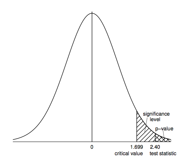
Why do we need two methods if they will always lead to the same decision? Well, when learning about hypothesis tests and becoming comfortable with their logic, many people find the rejection region method a little easier to apply. However, when we start to rely on statistical software for conducting hypothesis tests in later chapters of the book, we will find the p-value method easier to use. At this stage, when doing hypothesis test calculations by hand, it is helpful to use both the rejection region method and the p-value method to reinforce learning of the general concepts. This also provides a useful way to check our calculations since if we reach a different conclusion with each method we will know that we have made a mistake.
Lower-tail tests
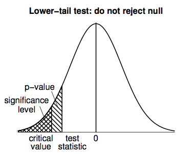
Lower-tail tests work in a similar way to upper-tail tests, but all the calculations are performed in the negative (left-hand) tail of the t-distribution density curve; the following figure illustrates.
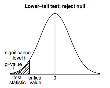
A lower-tail test would result in an inconclusive result for the home prices example (since the large, positive t-statistic means that the data favor neither the null hypothesis, NH: E(Y) = 255, nor the alternative hypothesis, AH: E(Y) < 255).
Two-tail tests
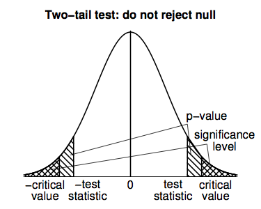
Two-tail tests work similarly, but we have to be careful to work with both tails of the t-distribution; the following figure illustrates.
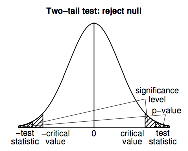
For the home prices example, we might want to do a two-tail hypothesis test if we had no prior expectation about how large or small sale prices are, but just wanted to see whether or not the realtor's claim of \(\$\)255,000 was plausible. The steps involved are as follows.
- State null hypothesis: NH: E(Y) = 255.
- State alternative hypothesis: AH: E(Y) ≠ 255.
- Calculate test statistic: t-statistic = \(m_Y−\text{E}(Y)/(s_Y/\sqrt{n})=(278.6033−255)/(53.8656/\sqrt{30})=2.40\).
- Set significance level: 5%.
- Look up t-table:
- critical value: The 97.5th percentile of the t-distribution with 29 degrees of freedom is 2.045; the rejection region is therefore any t-statistic greater than 2.045 or less than −2.045 (we need the 97.5th percentile in this case because this is a two-tail test, so we need half the significance level in each tail).
- p-value: The area to the right of the t-statistic (2.40) for the t-distribution with 29 degrees of freedom is less than 0.025 but greater than 0.01 (since the 97.5th percentile of this t-distribution is 2.045 and the 99th percentile is 2.462); thus the upper-tail area is between 0.01 and 0.025 and the two-tail p-value is twice as big as this, that is, between 0.02 and 0.05.
- Make decision:
- Since the t-statistic of 2.40 falls in the rejection region, we reject the null hypothesis in favor of the alternative.
- Since the p-value is between 0.02 and 0.05, it must be less than the significance level (0.05), so we reject the null hypothesis in favor of the alternative.
- Interpret in the context of the situation: The 30 sample sale prices suggest that a population mean of $255,000 seems implausible—the sample data favor a value different from this (at a significance level of 5%).
Hypothesis test errors
When we introduced the significance level above, we saw that the person conducting the hypothesis test gets to choose this value. We now explore this notion a little more fully. Whenever we conduct a hypothesis test, either we reject the null hypothesis in favor of the alternative or we do not reject the null hypothesis. "Not rejecting" a null hypothesis isn't quite the same as "accepting" it. All we can say in such a situation is that we do not have enough evidence to reject the null—recall the legal analogy where defendants are not found "innocent" but rather are found "not guilty." Anyway, regardless of the precise terminology we use, we hope to reject the null when it really is false and to "fail to reject it" when it really is true. Anything else will result in a hypothesis test error. There are two types of error that can occur, as illustrated in the following table:
| Decision | |||
| Do not reject NH in favor or AH | Reject NH in favor of AH | ||
| Reality | NH true | Correct decision | Type 1 error |
| NH false | Type 2 error | Correct decision | |
A type 1 error can occur if we reject the null hypothesis when it is really true—the probability of this happening is precisely the significance level. If we set the significance level lower, then we lessen the chance of a type 1 error occurring. Unfortunately, lowering the significance level increases the chance of a type 2 error occurring—when we fail to reject the null hypothesis but we should have rejected it because it was false. Thus, we need to make a trade-off and set the significance level low enough that type 1 errors have a low chance of happening, but not so low that we greatly increase the chance of a type 2 error happening. The default value of 5% tends to work reasonably well in many applications at balancing both goals. However, other factors also affect the chance of a type 2 error happening for a specific significance level. For example, the chance of a type 2 error tends to decrease the greater the sample size.

