Lesson 3: SLR Estimation & Prediction
Lesson 3: SLR Estimation & PredictionOverview
Typical regression analysis involves the following steps:
- Model formulation
- Model estimation
- Model evaluation
- Model use
So far, we have learned how to formulate and estimate a simple linear regression model. We have also learned about some model evaluation methods (and we will learn further evaluation methods in Lesson 4). In this lesson, we focus our efforts on using the model to answer two specific research questions, namely:
- What is the average response for a given value of the predictor x?
- What is the value of the response likely to be for a given value of the predictor x?
In particular, we will learn how to calculate and interpret:
- A confidence interval for estimating the mean response for a given value of the predictor x.
- A prediction interval for predicting a new response for a given value of the predictor x.
Objectives
- Distinguish between estimating a mean response (confidence interval) and predicting a new observation (prediction interval).
- Understand the factors that affect the width of a confidence interval for a mean response.
- Understand why a prediction interval for a new response is wider than the corresponding confidence interval for a mean response.
- Know the formula for a prediction interval depends strongly on the condition that the error terms are normally distributed, while the formula for the confidence interval is not so dependent on this condition for large samples.
- Know the types of research questions that can be answered using the materials and methods of this lesson.
Lesson 3 Code Files
Below is a zip file that contains all the data sets used in this lesson:
- skincancer.txt
- student_height_weight.txt
3.1 - The Research Questions
3.1 - The Research QuestionsIn this lesson, we are concerned with answering two different types of research questions. Our goal here — and throughout the practice of statistics — is to translate the research questions into reasonable statistical procedures.
Let's take a look at examples of the two types of research questions we learn how to answer in this lesson:
1. What is the mean weight, \(\mu\), of all American women, aged 18-24?
If we wanted to estimate \(\mu\), what would be a good estimate? It seems reasonable to calculate a confidence interval for \(\mu\) using \(\bar{y}\), the average weight of a random sample of American women, aged 18-24.
2. What is the weight, y, of an individual American woman, aged 18-24?
If we want to predict y, what would be a good prediction? It seems reasonable to calculate a "prediction interval" for y using, again, \(\bar{y}\), the average weight of a random sample of American women, aged 18-24.
A person's weight is, of course, highly associated with the person's height. In answering each of the above questions, we likely could do better by taking into account a person's height. That's where an estimated regression equation becomes useful.
Here are some weight and height data from a sample of n = 10 people, (Student Height and Weight data):
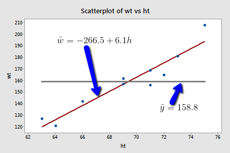
If we used the average weight of the 10 people in the sample to estimate \(\mu\), we would claim that the average weight of all American women aged 18-24 is 158.8 pounds regardless of the height of the women. Similarly, if we used the average weight of the 10 people in the sample to predict y, we would claim that the weight of an individual American woman aged 18-24 is 158.8 pounds regardless of the woman's height.
On the other hand, if we used the estimated regression equation to estimate \(\mu\), we would claim that the average weight of all American women aged 18-24 who are only 64 inches tall is -266.5 + 6.1(64) = 123.9 pounds. Similarly, we would predict that the weight y of an individual American woman aged 18-24 who is only 64 inches tall is 123.9 pounds. This example makes it clear that we get significantly different (and better!) answers to our research questions when we take into account a person's height.
Let's make it clear that it is one thing to estimate \(\mu_{Y}\)and yet another thing to predict y. (Note that we subscript \(\mu\) with Y to make it clear that we are talking about the mean of the response Y not the mean of the predictor x.)
Let's return to our example in which we consider the potential relationship between the predictor "high school GPA" and the response "college entrance test score."
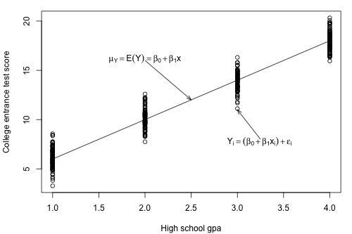
For this example, we could ask two different research questions concerning the response:
- What is the mean college entrance test score for the subpopulation of students whose high school GPA is 3? (Answering this question entails estimating the mean response \(\mu_{Y}\) when x = 3.)
- What college entrance test score can we predict for a student whose high school GPA is 3? (Answering this question entails predicting the response \(y_{\text{new}}\) when x = 3.)
The two research questions can be asked more generally:
- What is the mean response \(\mu_{Y}\) when the predictor value is \(x_{h}\)?
- What value will a new response \(y_{\text{new}}\) be when the predictor value is \(x_{h}\)?
Let's take a look at one more example, namely, the one concerning the relationship between the response "skin cancer mortality" and the predictor "latitude" (Skin Cancer data). Again, we could ask two different research questions concerning the response:
- What is the expected (mean) mortality rate due to skin cancer for all locations at 40 degrees north latitude?
- What is the predicted mortality rate for one individual location at 40 degrees north, say at Chambersburg, Pennsylvania?
At some level, answering these two research questions is straightforward. Both just involve using the estimated regression equation:
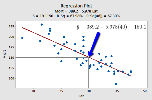
That is, \(\hat{y}_h=b_0+b_1x_h\) is the best answer to each research question. It is the best guess of the mean response at \(x_{h}\), and it is the best guess of a new response at \(x_{h}\):
- Our best estimate of the mean mortality rate due to skin cancer for all locations at 40 degrees north latitude is 389.19 - 5.97764(40) = 150 deaths per 10 million people.
- Our best prediction of the mortality rate due to skin cancer in Chambersburg, Pennsylvania is 389.19 - 5.97764(40) = 150 deaths per 10 million people.
The problem with the answers to our two research questions is that we'd have obtained a completely different answer if we had selected a different random sample of data. As always, to be confident in the answer to our research questions, we should put an interval around our best guesses. We learn how to do this in the next two sections. That is, we first learn a "confidence interval for \(\mu_Y\) " and then a "prediction interval for \(y_{\text{new}}\)."
Try It!
Research questions
For each of the following situations, identify whether the research question of interest entails estimating a mean response \(\mu_{Y}\) or predicting a new response \(y_{\text{new}}\).
3.2 - Confidence Interval for the Mean Response
3.2 - Confidence Interval for the Mean ResponseIn this section, we are concerned with the confidence interval, called a "t-interval," for the mean response \(\mu_{Y}\) when the predictor value is \(x_{h}\). Let's jump right in and learn the formula for the confidence interval. The general formula in words is as always:
Sample estimate ± (t-multiplier × standard error)
and the formula in notation is:
\(\hat{y}_h \pm t_{(1-\alpha/2, n-2)} \times \sqrt{MSE \times \left( \frac{1}{n} + \dfrac{(x_h-\bar{x})^2}{\sum(x_i-\bar{x})^2}\right)}\)
where:
- \(\hat{y}_h\) is the "fitted value" or "predicted value" of the response when the predictor is \(x_h\)
- \(t_{(1-\alpha/2, n-2)}\) is the "t-multiplier." Note that the t-multiplier has n-2 (not n-1) degrees of freedom because the confidence interval uses the mean square error (MSE) whose denominator is n-2.
- \(\sqrt{MSE \times \left( \frac{1}{n} + \frac{(x_h-\bar{x})^2}{\sum(x_i-\bar{x})^2}\right)}\) is the "standard error of the fit," which depends on the mean square error (MSE), the sample size (n), how far in squared units the predictor value \(x_h\) is from the average of the predictor values \(\bar{x}\), or \((x_h-\bar{x})^2\) , and the sum of the squared distances of the predictor values \(x_i\) from the average of the predictor values \(\bar{x}\), or \(\sum(x_i-\bar{x})^2\).
Fortunately, we won't have to use the formula to calculate the confidence interval in real-life practice, since statistical software such as Minitab will do the dirty work for us. Look at this Minitab output for our example with "skin cancer mortality" as the response and "latitude" as the predictor (Skin Cancer data):
Prediction for Mort
Regression Equation
Mort = 389.2 - 5.978 Lat
Settings
| Variable | Setting |
|---|---|
| Lat | 40 |
Prediction
| Fit | SE Fit | 95% CI | 95% PI |
|---|---|---|---|
| 150.084 | 2.74500 | (144.562, 155.606) | (111.235, 188.933) |
Here's what the output tells us:
- In the section labeled "Settings," Minitab reports the value \(x_{h}\) (40 degrees north) for which we requested the confidence interval for \(\mu_{Y}\).
- In the section labeled "Prediction," Minitab reports a 95% confidence interval. We can be 95% confident that the average skin cancer mortality rate of all locations at 40 degrees north is between 144.562 and 155.606 deaths per 10 million people.
- In the section labeled "Prediction," Minitab also reports the predicted value \(\hat{y}_h\), ("Fit" = 150.084), the standard error of the fit ("SE Fit" = 2.74500), and the 95% prediction interval for a new response (which we discuss in the next section).
Factors affecting the width of the t-interval for the mean response \(\mu_{Y}\)
Why do we bother learning the formula for the confidence interval for \(\mu_{Y}\) when we let statistical software calculate it for us anyway? As always, the formula is useful for investigating what factors affect the width of the confidence interval for \(\mu_{Y}\). Again, the formula is:
\(\hat{y}_h \pm t_{(1-\alpha/2, n-2)} \times \sqrt{MSE \times \left( \dfrac{1}{n} + \dfrac{(x_h-\bar{x})^2}{\sum(x_i-\bar{x})^2}\right)}\)
and therefore the width of the confidence interval for \(\mu_{Y}\) is:
\(2 \times \left(t_{(1-\alpha/2, n-2)} \times \sqrt{MSE \times \left( \dfrac{1}{n} + \dfrac{(x_h-\bar{x})^2}{\sum(x_i-\bar{x})^2}\right)}\right)\)
So how can we affect the width of our resulting interval for \(\mu_{Y}\)?
- As the mean square error (MSE) decreases, the width of the interval decreases. Since MSE is an estimate of how much the data vary naturally around the unknown population regression line, we have little control over MSE other than making sure that we make our measurements as carefully as possible. (We will return to this issue later in the course when we address "model selection.")
- As we decrease the confidence level, the t-multiplier decreases, and hence the width of the interval decreases. In practice, we wouldn't want to set the confidence level below 90%.
- As we increase the sample size n, the width of the interval decreases. We have complete control over the size of our sample — the only limitation being our time and financial constraints.
- The more spread out the predictor values, the larger the quantity \(\sum(x_i-\bar{x})^2\) and hence the narrower the interval. In general, you should make sure your predictor values are not too clumped together but rather sufficiently spread out.
- The closer \(x_{h}\) is to the average of the sample's predictor values \(\bar{x}\), the smaller the quantity \((x_h-\bar{x})^2\), and hence the narrower the interval. If you know that you want to use your estimated regression equation to estimate \(\mu_{Y}\) when the predictor's value is \(x_{h}\), then you should be aware that the confidence interval will be narrower the closer \(x_{h}\) is to \(\bar{x}\).
Let's see this last claim in action for our example with "skin cancer mortality" as the response and "latitude" as the predictor:
Settings
| New Obs | Latitude |
|---|---|
| 1 | 40.0 |
| 2 | 28.0 |
Predictions
| New | Fit | SE Fit | 95.0% CI | 95.0% PI |
|---|---|---|---|---|
| 1 | 150.08 | 2.75 | (144.6, 155.6) | (111.2, 188.93) |
| 2 | 221.82 | 7.42 | (206.9, 236.8) | (180.6, 263.07) X |
| X Denotes an unusual point relative to predictor levels used to fit the model | ||||
Mean of Lat 39.533
The Minitab output reports a 95% confidence interval for \(\mu_{Y}\) for a latitude of 40 degrees north (first row) and 28 degrees north (second row). The average latitude of the 49 states in the data set is 39.533 degrees north. The output tells us:
- We can be 95% confident that the mean skin cancer mortality rate of all locations at 40 degrees north is between 144.6 and 155.6 deaths per 10 million people.
- And, we can be 95% confident that the mean skin cancer mortality rate of all locations at 28 degrees north is between 206.9 and 236.8 deaths per 10 million people.
The width of the 40-degree north interval (155.6 - 144.6 = 11 deaths) is shorter than the width of the 28-degree north interval (236.8 - 206.9 = 29.9 deaths), because 40 is much closer than 28 is to the sample mean 39.533. Note that Minitab is kind enough to warn us ("X denotes an unusual point relative to predictor levels used to fit the model") that 28 degrees north is far from the mean of the sample's predictor values.
When is it okay to use the formula for the confidence interval for \(\mu_{Y}\)?
One thing we haven't discussed yet is when it is okay to use the formula for the confidence interval for \(\mu_{Y}\). It is okay:
- When \(x_{h}\) is a value within the range of the x values in the data set — that is when \(x_{h}\) is a value within the "scope of the model." But, note that \(x_{h}\) does not have to be one of the actual x values in the data set.
- When the "LINE" conditions — linearity, independent errors, normal errors, equal error variances — are met. The formula works okay even if the error terms are only approximately normal. And, if you have a large sample, the error terms can even deviate substantially from normality.
3.3 - Prediction Interval for a New Response
3.3 - Prediction Interval for a New ResponseIn this section, we are concerned with the prediction interval for a new response, \(y_{new}\), when the predictor's value is \(x_h\). Again, let's just jump right in and learn the formula for the prediction interval. The general formula in words is as always:
Sample estimate ± (t-multiplier × standard error)
and the formula in notation is:
\(\hat{y}_h \pm t_{(1-\alpha/2, n-2)} \times \sqrt{MSE \times \left(1+ \frac{1}{n} + \dfrac{(x_h-\bar{x})^2}{\sum(x_i-\bar{x})^2}\right)}\)
where:
- \(\hat{y}_h\) is the "fitted value" or "predicted value" of the response when the predictor is \(x_h\)
- \(t_{(1-\alpha/2, n-2)}\) is the "t-multiplier." Note again that the t-multiplier has n-2 (not n-1) degrees of freedom because the prediction interval uses the mean square error (MSE) whose denominator is n-2.
- \(\sqrt{MSE \times \left(1+ \frac{1}{n} + \frac{(x_h-\bar{x})^2}{\sum(x_i-\bar{x})^2}\right)}\) is the "standard error of the prediction," which is very similar to the "standard error of the fit" when estimating \(\mu_Y\). The standard error of the prediction just has an extra MSE term added that the standard error of the fit does not. (More on this a bit later.)
Again, we won't use the formula to calculate our prediction intervals in real-life practice. We'll let statistical software such as Minitab do the calculations for us. Let's look at the prediction interval for our example with "skin cancer mortality" as the response and "latitude" as the predictor (Skin Cancer data):
Prediction for Mort
Regression Equation
Mort = 389.2 - 5.978 Lat
Settings
| Variable | Setting |
|---|---|
| Lat | 40 |
Prediction
| Fit | SE Fit | 95% CI | 95% PI |
|---|---|---|---|
| 150.084 | 2.74500 | (144.562, 155.606) | (111.235, 188.933) |
The output reports the 95% prediction interval for an individual location at 40 degrees north. We can be 95% confident that the skin cancer mortality rate at an individual location at 40 degrees north is between 111.235 and 188.933 deaths per 10 million people.
When is it okay to use the prediction interval for the \(y_{new}\) formula?
The requirements are similar to, but a little more restrictive than those for the confidence interval. It is okay:
- When \(x_{h}\) is a value within the scope of the model. Again, \(x_{h}\) does not have to be one of the actual x values in the data set.
- When the "LINE" conditions — linearity, independent errors, normal errors, equal error variances — are met. Unlike the case for the formula for the confidence interval, the formula for the prediction interval depends strongly on the condition that the error terms are normally distributed.
Understanding the difference in the two formulas
In our discussion of the confidence interval for \(\mu_{Y}\), we used the formula to investigate what factors affect the width of the confidence interval. There's no need to do it again. Because the formulas are so similar, it turns out that the factors affecting the width of the prediction interval are identical to the factors affecting the width of the confidence interval.
Let's instead investigate the formula for the prediction interval for \(y_{new}\):
\(\hat{y}_h \pm t_{(1-\alpha/2, n-2)} \times \sqrt{MSE \times \left( 1+\dfrac{1}{n} + \dfrac{(x_h-\bar{x})^2}{\sum(x_i-\bar{x})^2}\right)}\)
to see how it compares to the formula for the confidence interval for \(\mu_{Y}\):
\(\hat{y}_h \pm t_{(1-\alpha/2, n-2)} \times \sqrt{MSE \left(\dfrac{1}{n} + \dfrac{(x_h-\bar{x})^2}{\sum(x_i-\bar{x})^2}\right)}\)
Observe that the only difference in the formulas is that the standard error of the prediction for \(y_{new}\) has an extra MSE term in it that the standard error of the fit for \(\mu_{Y}\) does not.
Let's try to understand the prediction interval to see what causes the extra MSE term. In doing so, let's start with an easier problem first. Think about how we could predict a new response \(y_{new}\) at a particular \(x_{h}\) if the mean of the responses \(\mu_{Y}\) at \(x_{h}\) were known. That is, suppose it was known that the mean skin cancer mortality at \(x_{h} = 40^{o}\) N is 150 deaths per million (with variance 400)? What is the predicted skin cancer mortality in Columbus, Ohio?
Because \(\mu_{Y} = 150 \) and \( \sigma^{2} = 400\) are known, we can take advantage of the "empirical rule," which states among other things that 95% of the measurements of normally distributed data are within 2 standard deviations of the mean. That is, it says that 95% of the measurements are in the interval sandwiched by:
\(\mu_{Y}- 2\sigma\) and \(\mu_{Y}+ 2\sigma\).
Applying the 95% rule to our example with \(\mu_{Y} = 150\) and \(\sigma= 20\):
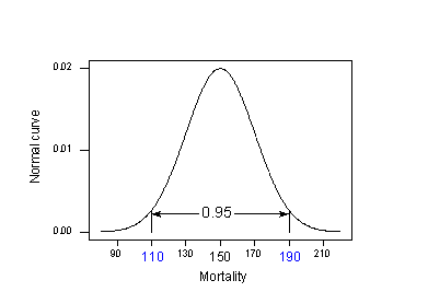
95% of the skin cancer mortality rates of locations at 40 degrees north latitude are in the interval sandwiched by:
150 - 2(20) = 110 and 150 + 2(20) = 190.
That is, if someone wanted to know the skin cancer mortality rate for a location at 40 degrees north, our best guess would be somewhere between 110 and 190 deaths per 10 million. The problem is that our calculation used \(\mu_{Y}\) and \(\sigma\), population values that we would typically not know. Reality sets in:
- The mean \(\mu_{Y}\) is typically not known. The logical thing to do is estimate it with the predicted response \(\hat{y}\). The cost of using \(\hat{y}\) to estimate \(\mu_{Y}\) is the variance of \(\hat{y}\). That is, different samples would yield different predictions \(\hat{y}\), and so we have to take into account this variance of \(\hat{y}\).
- The variance \( \sigma^{2}\) is typically not known. The logical thing to do is to estimate it with MSE.
Because we have to estimate these unknown quantities, the variation in the prediction of a new response depends on two components:
- The variation due to estimating the mean \(\mu_{Y}\) with \(\hat{y}_h\) , which we denote "\(\sigma^2(\hat{Y}_h)\)."(Note that the estimate of this quantity is just the square of the standard error of the fit that appears in the confidence interval formula.)
- The variation in the responses y, which we denote as "\(\sigma^2\)."(Note that quantity is estimated, as usual, with the mean square error MSE.)
Adding the two variance components, we get:
\(\sigma^2+\sigma^2(\hat{Y}_h)\)
which is estimated by:
\(MSE+MSE \left( \dfrac{1}{n} + \dfrac{(x_h-\bar{x})^2}{\sum_{i=1}^{n}(x_i-\bar{x})^2} \right) =MSE\left( 1+\dfrac{1}{n} + \dfrac{(x_h-\bar{x})^2}{\sum_{i=1}^{n}(x_i-\bar{x})^2} \right) \)
Do you recognize this quantity? It's just the variance of the prediction that appears in the formula for the prediction interval \(y_{new}\)!
Let's compare the two intervals again:
Confidence interval for \(\mu_{Y}\colon \hat{y}_h \pm t_{(1-\alpha/2, n-2)} \times \sqrt{MSE \times \left( \frac{1}{n} + \frac{(x_h-\bar{x})^2}{\sum(x_i-\bar{x})^2}\right)}\)
Prediction interval for \(y_{new}\colon \hat{y}_h \pm t_{(1-\alpha/2, n-2)} \times \sqrt{MSE \left( 1+\frac{1}{n} + \frac{(x_h-\bar{x})^2}{\sum(x_i-\bar{x})^2}\right)}\)
What are the practical implications of the difference between the two formulas?
- Because the prediction interval has the extra MSE term, a \( \left( 1-\alpha \right) 100\% \) confidence interval for \(\mu_{Y}\) at \(x_{h}\) will always be narrower than the corresponding \( \left( 1-\alpha \right) 100\% \) prediction interval for \(y_{new}\) at \(x_{h}\).
- By calculating the interval at the sample's mean of the predictor values \(\left(x_{h} = \bar{x}\right)\) and increasing the sample size n, the confidence interval's standard error can approach 0. Because the prediction interval has the extra MSE term, the prediction interval's standard error cannot get close to 0.
The first implication is seen most easily by studying the following plot for our skin cancer mortality example:
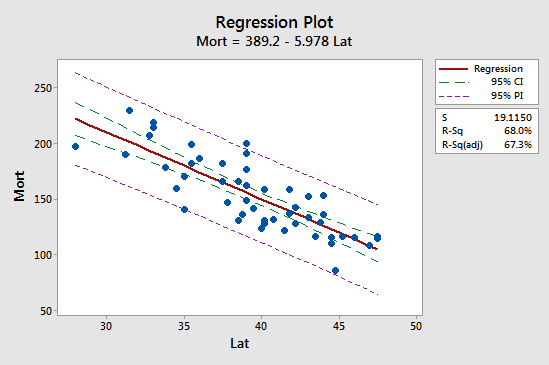
Observe that the prediction interval (95% PI, in purple) is always wider than the confidence interval (95% CI, in green). Furthermore, both intervals are narrowest at the mean of the predictor values (about 39.5).
3.4 - Further Example
3.4 - Further ExampleExample 3-1: Hospital Infection Data

The hospital infection risk dataset consists of a sample of n = 58 hospitals in the east and north-central U.S. (Hospital Infection Data Region 1 and 2 data). The response variable is y = infection risk (percent of patients who get an infection) and the predictor variable is x = average length of stay (in days). Minitab output for a simple linear regression model fit to these data follows:
Regression Analysis: InfctRsk versus Stay
Analysis of Variance
| Source | DF | Adj SS | Adj Ms | F-Value | P-Value |
|---|---|---|---|---|---|
| Regression | 1 | 38.3059 | 38.3059 | 36.50 | 0.000 |
| Stay | 1 | 38.3059 | 38.3059 | 36.50 | 0.000 |
| Error | 56 | 58.7763 | 1.0496 | ||
| Lack-of-Fit | 54 | 58.5513 | 1.0843 | 9.64 | 0.098 |
| Pure error | 2 | 0.2250 | 0.1125 | ||
| Total | 57 | 97.0822 |
Model Summary
| S | R-Sq | R-Sq (adj) | R-Sq (pred) |
|---|---|---|---|
| 1.02449 | 39.46% | 38.38% | 35.07% |
Coefficients
| Term | Coef | SE Coef | T-Value | P-Value | VIF |
|---|---|---|---|---|---|
| Constant | -1.160 | 0.956 | -1.21 | 0.230 | |
| Stay | 0.5689 | 0.0942 | 6.04 | 0.000 | 1.00 |
Regression Equation
InfctRsk = -1.160 + 0.5689 Stay
Minitab output with information for x = 10.
Prediction for InfctRsk
Regression Equation
InfctRsk = -1.160 + 0.5689 Stay
| Variable | Setting |
|---|---|
| Stay | 10 |
| Fit | SE Fit | 95% CI | 95% PI |
|---|---|---|---|
| 4.52885 | 0.134602 | (4.25921, 4.79849) | (2.45891, 6.59878) |
We can make the following observations:
- For the interval given under 95% CI, we say with 95% confidence we can estimate that in hospitals in which the average length of stay is 10 days, the mean infection risk is between 4.25921 and 4.79849.
- For the interval given under 95% PI, we say with 95% confidence that for any future hospital where the average length of stay is 10 days, the infection risk is between 2.45891 and 6.59878.
- The value under Fit is calculated as \(\hat{y} = −1.160 + 0.5689(10) = 4.529\).
- The value under SE Fit is the standard error of \(\hat{y}\) and it measures the accuracy of \(\hat{y}\) as an estimate of E(Y ).
- Since df = n − 2 = 58 − 2 = 56, the multiplier for 95% confidence is 2.00324. The 95% CI for E(Y) is calculated as \begin{align} &=4.52885 \pm (2.00324 × 0.134602)\\ &= 4.52885 \pm 0.26964\\ &= (4.259, 4.798)\end{align}
- Since S = \(\sqrt{MSE}\) = 1.02449, the 95% PI is calculated as \begin{align} &=4.52885 \pm (2.00324 × \sqrt{1.02449^2 + 0.134602^2})\\ &= 4.52885 \pm 2.0699 = (2.459, 6.599)\end{align}
The following figure provides plots showing the difference between the confidence intervals (CI) and prediction intervals (PI) we have been considering.

There are also some things to note:
- Notice that the limits for E(Y) are close to the line. The purpose of those limits is to estimate the "true" location of the line.
- Notice that the prediction limits (on the right) bracket most of the data. Those limits describe the location of individual y-values.
- Notice that the prediction intervals are wider than the confidence intervals. This is something that can be noted by the formulas.
Software Help 3
Software Help 3
The next two pages cover the Minitab and R commands for the procedures in this lesson.
Below is a zip file that contains all the data sets used in this lesson:
- skincancer.txt
- student_height_weight.txt
Minitab Help 3: SLR Estimation & Prediction
Minitab Help 3: SLR Estimation & PredictionMinitab® – Help
Student heights and weights
- Perform a basic regression analysis with y = wt and x = ht.
- Create a fitted line plot.
- Use Editor > Add > Reference Lines to add a horizontal line at the mean weight.
- Find a confidence interval and a prediction interval for the response to predict weight for height = 64.
Skin cancer mortality
- Perform a basic regression analysis with y = Mort and x = Lat.
- Create a fitted line plot.
- Find a confidence interval and a prediction interval for the response to calculate 95% confidence intervals for E(Mort) at Lat = 40 and 28.
- Calculate mean(Lat).
- Find a confidence interval and a prediction interval for the response to calculate a 95% prediction interval for Mort at Lat = 40.
- Create a fitted line plot with confidence bands and prediction bands.
Hospital infection risk
- Use Data > Subset Worksheet to select only hospitals in regions 1 or 2.
- Create a basic scatterplot of Stay versus InfctRsk.
- Use Data > Subset Worksheet to select only hospitals with Stay < 16 (i.e., remove the two hospitals with extreme values of Stay).
- Perform a basic regression analysis with y = InfctRsk and x = Stay.
- Find a confidence interval and a prediction interval for the response to calculate 95% confidence intervals for E(InfctRsk) at Stay = 10 and 95% prediction intervals for InfctRsk at Stay = 10.
- Create a fitted line plot with confidence bands and prediction bands
R Help 3: SLR Estimation & Prediction
R Help 3: SLR Estimation & PredictionR Help
Student heights and weights
- Load the heightweight data.
- Fit a simple linear regression model with y = wt and x = ht.
- Display a scatterplot of the data with the simple linear regression line and a horizontal line at the mean weight.
- Use the model to predict weight for height = 64.
heightweight <- read.table("~/path-to-folder/student_height_weight.txt", header=T)
attach(heightweight)

model <- lm(wt ~ ht)
plot(x=ht, y=wt,
     panel.last = c(lines(sort(ht), fitted(model)[order(ht)]),
                    abline(h=mean(wt))))
mean(wt) # 158.8
predict(model, newdata=data.frame(ht=64)) # 126.2708

detach(heightweight)
Skin cancer mortality
- Load the skin cancer data.
- Fit a simple linear regression model with y = Mort and x = Lat.
- Display a scatterplot of the data with the simple linear regression line.
- Use the model to calculate 95% confidence intervals for E(Mort) at Lat = 40 and 28.
- Calculate mean(Lat).
- Use the model to calculate 95% prediction intervals for Mort at Lat = 40.
- Display a scatterplot of the data with the simple linear regression line, confidence interval bounds, and prediction interval bounds.
skincancer <- read.table("~/path-to-folder/skincancer.txt", header=T)
attach(skincancer)

model <- lm(Mort ~ Lat)
plot(x=Lat, y=Mort,
     xlab="Latitude (at center of state)", ylab="Mortality (deaths per 10 million)",
     main="Skin Cancer Mortality versus State Latitude",
     panel.last = lines(sort(Lat), fitted(model)[order(Lat)]))

predict(model, interval="confidence", se.fit=T,
        newdata=data.frame(Lat=c(40, 28)))
# $fit
#        fit      lwr      upr
# 1 150.0839 144.5617 155.6061
# 2 221.8156 206.8855 236.7456
#
# $se.fit
# 1        2
# 2.745000 7.421459

mean(Lat) # 39.53265

predict(model, interval="prediction",
        newdata=data.frame(Lat=40))
#        fit     lwr      upr
# 1 150.0839 111.235 188.9329

plot(x=Lat, y=Mort,
     xlab="Latitude (at center of state)", ylab="Mortality (deaths per 10 million)",
     ylim=c(60, 260),
     panel.last = c(lines(sort(Lat), fitted(model)[order(Lat)]),
                    lines(sort(Lat),
                          predict(model,
                                  interval="confidence")[order(Lat), 2], col="green"),
                    lines(sort(Lat),
                          predict(model,
                                  interval="confidence")[order(Lat), 3], col="green"),
                    lines(sort(Lat),
                          predict(model,
                                  interval="prediction")[order(Lat), 2], col="purple"),
                    lines(sort(Lat),
                          predict(model,
                                  interval="prediction")[order(Lat), 3], col="purple")))

detach(skincancer)
Hospital infection risk
- Load the infectionrisk data.
- Select only hospitals in regions 1 or 2.
- Display a scatterplot of Stay versus InfctRsk.
- Select only hospitals with Stay < 16 (i.e., remove the two hospitals with extreme values of Stay).
- Fit a simple linear regression model with y = InfctRsk and x = Stay.
- Use the model to calculate 95% confidence intervals for E(InfctRsk) at Stay = 10.
- Use the model to calculate 95% prediction intervals for InfctRsk at Stay = 10.
- Display a scatterplot of the data with the simple linear regression line, confidence interval bounds, and prediction interval bounds.
infectionrisk <- read.table("~/path-to-folder/infectionrisk.txt", header=T)
infectionrisk <- infectionrisk[infectionrisk$Region==1 | infectionrisk$Region==2, ]
attach(infectionrisk)
plot(x=Stay, y=InfctRsk)
detach(infectionrisk)
infectionrisk <- infectionrisk[infectionrisk$Stay<16, ]
attach(infectionrisk)
plot(x=Stay, y=InfctRsk)

model <- lm(InfctRsk ~ Stay)

predict(model, interval="confidence",
        newdata=data.frame(Stay=10))
#        fit      lwr      upr
# 1 4.528846 4.259205 4.798486

predict(model, interval="prediction",
        newdata=data.frame(Stay=10))
#        fit     lwr      upr
# 1 4.528846 2.45891 6.598781

plot(x=Stay, y=InfctRsk,
     ylim=c(0, 9),
     panel.last = c(lines(sort(Stay), fitted(model)[order(Stay)]),
                    lines(sort(Stay),
                          predict(model,
                                  interval="confidence")[order(Stay), 2], col="green"),
                    lines(sort(Stay),
                          predict(model,
                                  interval="confidence")[order(Stay), 3], col="green"),
                    lines(sort(Stay),
                          predict(model,
                                  interval="prediction")[order(Stay), 2], col="purple"),
                    lines(sort(Stay),
                          predict(model,
                                  interval="prediction")[order(Stay), 3], col="purple")))

detach(infectionrisk)