Lesson 7: MLR Estimation, Prediction & Model Assumptions
Lesson 7: MLR Estimation, Prediction & Model AssumptionsOverview
This lesson extends the methods from Lesson 3 and Lesson 4 to the context of multiple linear regression. Thus, we focus our efforts on using a multiple linear regression model to answer two specific research questions, namely:
- What is the average response for a given set of values of the predictors \(x_1 , x_2 \dots \text{?}\)
- What is the value of the response likely to be for a given set of values of the predictors \(x_1, x_2 \dots \text{?}\)
In particular, we will learn how to calculate and interpret:
- A confidence interval for estimating the mean response for a given set of values of the predictors \(x_1, x_2 \dots\)
- A prediction interval for predicting a new response for a given set of values of the predictors \(x_1, x_2 \dots\)
How do we evaluate a model? How do we know if the model we are using is good? One way to consider these questions is to assess whether the assumptions underlying the multiple linear regression model seem reasonable when applied to the dataset in question. Since the assumptions relate to the (population) prediction errors, we do this by studying the (sample) estimated errors, the residuals.
Objectives
- Distinguish between estimating a mean response (confidence interval) and predicting a new observation (prediction interval).
- Understand the various factors that affect the width of a confidence interval for a mean response.
- Understand why a prediction interval for a new response is wider than the corresponding confidence interval for a mean response.
- Know the formula for a prediction interval depends strongly on the condition that the error terms are normally distributed, while the formula for the confidence interval is not so dependent on this condition for large samples.
- Know the types of research questions that can be answered using the materials and methods of this lesson.
- Understand why we need to check the assumptions of our model.
- Know the things that can go wrong with the linear regression model.
- Know how we can detect various problems with the model using a residuals vs. fits plot.
- Know how we can detect various problems with the model using a residuals vs. predictor plot.
- Know how we can detect a certain kind of dependent error terms using a residuals vs. order plot.
- Know how we can detect non-normal error terms using a normal probability plot.
- Apply some numerical tests for assessing model assumptions.
Lesson 7 Code Files
Below is a text file that contains the data used in this lesson:
7.1 - Confidence Interval for the Mean Response
7.1 - Confidence Interval for the Mean ResponseIn this section, we are concerned with the confidence interval, called a "t-interval," for the mean response μY when the predictor values are \(\textbf{X}_{h}=(1, X_{h,1}, X_{h,2}, \dots, X_{h,p-1})^\textrm{T}\). The general formula in words is as always:
Sample estimate ± (t-multiplier × standard error)
First, we define the standard error of the fit at \(\textbf{X}_{h}\) given by:
\(\textrm{se}(\hat{y}_{h})=\sqrt{\textrm{MSE}(\textbf{X}_{h}^{\textrm{T}}(\textbf{X}^{\textrm{T}}\textbf{X})^{-1}\textbf{X}_{h})}.\)
and the confidence interval is:
\(\hat{y}_h \pm t_{(1-\alpha/2, n-p)} \times \textrm{se}(\hat{y}_{h})\)
where:
- \(\hat{y}_h\) is the "fitted value" or "predicted value" of the response when the predictor values are \(\textbf{X}_{h}\).
- \(t_{(1-\alpha/2, n-p)}\) is the "t-multiplier." Note that the t-multiplier has n-p degrees of freedom because the confidence interval uses the mean square error (MSE) whose denominator is n-p.
Fortunately, we won't have to use the formula to calculate the confidence interval, since statistical software such as Minitab will do the dirty work for us. Here is some Minitab output for the example on IQ and physical characteristics from Lesson 5 (IQ Size data), where we've fit a model with PIQ as the response and Brain and Height as the predictors:
Settings
| New Obs | Brain | Height |
|---|---|---|
| 1 | 90.0 | 70.0 |
Prediction
| New Obs | Fit | SE Fit | 95% CI | 95% PI |
|---|---|---|---|---|
| 1 | 105.64 | 3.65 | (98.24, 113.04) | (65.35, 145.93) |
Here's what the output tells us:
- In the section labeled "Settings," Minitab reports the values for \(\textbf{X}_{h}\) (brain size = 90 and height = 70) for which we requested the confidence interval for \(\mu_{Y}\).
- In the section labeled "Prediction," Minitab reports a 95% confidence interval. We can be 95% confident that the average performance IQ score of all college students with brain size = 90 and height = 70 is between 98.24 and 113.04.
- In the section labeled "Prediction," Minitab also reports the predicted value \(\hat{y}_h\), ("Fit" = 105.64), the standard error of the fit ("SE Fit" = 3.65), and the 95% prediction interval for a new response (which we discuss in the next section).
Factors affecting the width of the t-interval for the mean response \(\left(\mu_{Y}\right)\)
As always, the formula is useful for investigating what factors affect the width of the confidence interval for \(\mu_{Y}\).
- As the mean square error (MSE) decreases, the width of the interval decreases. Since MSE is an estimate of how much the data vary naturally around the unknown population regression hyperplane, we have little control over MSE other than making sure that we make our measurements as carefully as possible.
- As we decrease the confidence level, the t-multiplier decreases, and hence the width of the interval decreases. In practice, we wouldn't want to set the confidence level below 90%.
- As we increase the sample size n, the width of the interval decreases. We have complete control over the size of our sample — the only limitation being our time and financial constraints.
- The closer \(\textbf{X}_{h}\) is to the average of the sample's predictor values, the narrower the interval.
Let's see this last claim in action for our IQ example:
Settings
| New Obs | Brain | Height |
|---|---|---|
| 1 | 79.0 | 62.0 |
Prediction
| New Obs | Fit | SE Fit | 95% CI | 95% PI |
|---|---|---|---|---|
| 1 | 104.81 | 6.60 | (91.42, 118.20) | (63.00, 146.62) |
The width of the first confidence interval we calculated earlier (113.04 - 98.24 = 14.80) is shorter than the width of this new interval (118.20 - 91.42 = 26.78), because 90 and 70 are much closer than 79 and 62 are to the sample means (90.7 and 68.4).
When is it okay to use the formula for the confidence interval for \(\mu_{Y}\) ?
- When \(\textbf{X}_{h}\) is within the "scope of the model." But, note that \(\textbf{X}_{h}\) does not have to be an actual observation in the data set.
- When the "LINE" conditions — linearity, independent errors, normal errors, equal error variances — are met. The formula works okay even if the error terms are only approximately normal. And, if you have a large sample, the error terms can even deviate substantially from normality.
7.2 - Prediction Interval for a New Response
7.2 - Prediction Interval for a New ResponseIn this section, we are concerned with the prediction interval for a new response \(y_{new}\) when the predictor values are \(\textbf{X}_{h}=(1, X_{h,1}, X_{h,2}, \dots, X_{h,p-1})^\textrm{T}\). Again, let's just jump right in and learn the formula for the prediction interval. The general formula in words is as always:
Sample estimate ± (t-multiplier × standard error)
and the formula in notation is:
\(\hat{y}_h \pm t_{(1-\alpha/2, n-p)} \times \sqrt{MSE + (\textrm{se}(\hat{y}_{h}))^2}\)
where:
- \(\hat{y}_h\) is the "fitted value" or "predicted value" of the response when the predictor values are \(\textbf{X}_{h}\).
- \(t_{(1-\alpha/2, n-p)}\) is the "t-multiplier." Note again that the t-multiplier has n-p degrees of freedom because the prediction interval uses the mean square error (MSE) whose denominator is n-p.
- \(\sqrt{MSE + (\textrm{se}(\hat{y}_{h}))^2}\) is the "standard error of the prediction," which is very similar to the "standard error of the fit" when estimating \(\mu_{Y}\). The standard error of the prediction just has an extra MSE term added that the standard error of the fit does not. (More on this a bit later.)
Again, we won't use the formula to calculate our prediction intervals. We'll let statistical software such as Minitab do the calculation for us. Let's look at the prediction interval for our IQ example (IQ Size data):
Settings
| New Obs | Brain | Height |
|---|---|---|
| 1 | 90.0 | 70.0 |
Prediction
| New Obs | Fit | SE Fit | 95% CI | 95% PI |
|---|---|---|---|---|
| 1 | 105.64 | 3.65 | (98.24, 113.04) | (65.35, 145.93) |
The output reports the 95% prediction interval for an individual college student with brain size = 90 and height = 70. We can be 95% confident that the performance IQ score of an individual college student with brain size = 90 and height = 70 will be between 65.35 and 145.93.
When is it okay to use the prediction interval for \(y_{new}\) formula?
The requirements are similar to, but a little more restrictive than, those for the confidence interval. It is okay:
- When \(\textbf{X}_{h}\) is within the "scope of the model." Again, \(\textbf{X}_{h}\) does not have to be an actual observation in the data set.
- When the "LINE" conditions — linearity, independent errors, normal errors, equal error variances — are met. Unlike the case for the formula for the confidence interval, the formula for the prediction interval depends strongly on the condition that the error terms are normally distributed.
Understanding the difference between the two formulas
In our discussion of the confidence interval for \(\mu_{Y}\), we used the formula to investigate what factors affect the width of the confidence interval. There's no need to do it again. Because the formulas are so similar, it turns out that the factors affecting the width of the prediction interval are identical to the factors affecting the width of the confidence interval.
Let's instead investigate the formula for the prediction interval for \(y_{new}\):
\(\hat{y}_h \pm t_{(\alpha/2, n-p)} \times \sqrt{MSE + (\textrm{se}(\hat{y}_{h}))^2}\)
to see how it compares to the formula for the confidence interval for \(\mu_{Y}\):
\(\hat{y}_h \pm t_{(\alpha/2, n-p)} \times \textrm{se}(\hat{y}_{h})\)
Observe that the only difference in the formulas is that the standard error of the prediction for \(y_{new}\) has an extra MSE term in it that the standard error of the fit for \(\mu_{Y}\) does not. If you're not sure why this makes sense, re-read Section 3.3 on "Prediction Interval for a New Response" in the context of simple linear regression.
What are the practical implications of the difference between the two formulas?
- Because the prediction interval has the extra MSE term, a \(\left(1-\alpha \right)100\%\) confidence interval for \(\mu_{Y}\) at \(\textbf{X}_{h}\) will always be narrower than the corresponding (1-α)100% prediction interval for \(y_{new}\) at \(\textbf{X}_{h}\).
- By calculating the interval at the sample means of the predictor values and increasing the sample size n, the confidence interval's standard error can approach 0. Because the prediction interval has the extra MSE term, the prediction interval's standard error cannot get close to 0.
7.3 - MLR Model Assumptions
7.3 - MLR Model AssumptionsThe four conditions ("LINE") that comprise the multiple linear regression model generalize the simple linear regression model conditions to take account of the fact that we now have multiple predictors:
- Linear Function: The mean of the response, \(\mbox{E}(Y_i)\), at each set of values of the predictors, \((x_{1i}, x_{2i},...)\), is a Linear function of the predictors.
- Independent: The errors, \( \epsilon_{i}\), are Independent.
- Normally Distributed: The errors, \( \epsilon_{i}\), at each set of values of the predictors, \((x_{1i}, x_{2i},...)\), are Normally distributed.
- Equal variances (denoted \(\sigma^{2}\)): The errors, \( \epsilon_{i}\), at each set of values of the predictors, \((x_{1i}, x_{2i},...)\), have Equal variances (denoted \(\sigma^{2}\)).
An equivalent way to think of the first (linearity) condition is that the mean of the error, \(\epsilon_i\), at each set of values of the predictors, \((x_{1i},x_{2i},\dots)\), is zero. An alternative way to describe all four assumptions is that the errors, \(\epsilon_i\), are independent normal random variables with mean zero and constant variance, \(\sigma^2\).
As in simple linear regression, we can assess whether these conditions seem to hold for a multiple linear regression model applied to a particular sample dataset by looking at the estimated errors, i.e., the residuals, \(e_i = y_i-\hat{y}_i\).
7.4 - Assessing the Model Assumptions
7.4 - Assessing the Model AssumptionsWe can use all the methods we learned about in Lesson 4 to assess the multiple linear regression model assumptions:
- Create a scatterplot with the residuals, \(e_i\), on the vertical axis and the fitted values, \(\hat{y}_i\), on the horizontal axis and visual assess whether:
- the (vertical) average of the residuals remains close to 0 as we scan the plot from left to right (this affirms the "L" condition);
- the (vertical) spread of the residuals remains approximately constant as we scan the plot from left to right (this affirms the "E" condition);
- there are no excessively outlying points (we'll explore this in more detail in Lesson 11).
- violation of any of these three may necessitate remedial action (such as transforming one or more predictors and/or the response variable), depending on the severity of the violation (we'll explore this in more detail in Lesson 9).
- If the data observations were collected over time (or space) create a scatterplot with the residuals, \(e_i\), on the vertical axis and the time (or space) sequence on the horizontal axis and visual assess whether there is no systematic non-random pattern (this affirms the "I" condition).
- Violation may suggest the need for a time series model (see the optional content).
- Create a series of scatterplots with the residuals, \(e_i\), on the vertical axis and each of the predictors in the model on the horizontal axes and visually assess whether:
- the (vertical) average of the residuals remains close to 0 as we scan the plot from left to right (this affirms the "L" condition);
- the (vertical) spread of the residuals remains approximately constant as we scan the plot from left to right (this affirms the "E" condition);
- violation of either of these for at least one residual plot may suggest the need for transformations of one or more predictors and/or the response variable (again we'll explore this in more detail in Lesson 9).
- Create a histogram, boxplot, and/or normal probability plot of the residuals, \(e_i\) to check for approximate normality (the "N" condition). (Of these plots, the normal probability plot is generally the most effective.)
- Create a series of scatterplots with the residuals, \(e_i\), on the vertical axis and each of the available predictors that have been omitted from the model on the horizontal axes and visually assess whether:
- there are no strong linear or simple nonlinear trends in the plot;
- violation may indicate the predictor in question (or a transformation of the predictor) might be usefully added to the model.
- it can sometimes be helpful to plot functions of predictor variables on the horizontal axis of a residual plot, for example, interaction terms consisting of one quantitative predictor multiplied by another quantitative predictor. A strong linear or simple nonlinear trend in the resulting plot may indicate the variable plotted on the horizontal axis might be usefully added to the model.
As you can see, checking the assumptions for a multiple linear regression model comprehensively is not a trivial undertaking! But, the more thorough we are in doing this, the greater the confidence we can have in our model. To illustrate, let's do a residual analysis for the example on IQ and physical characteristics from Lesson 5 (IQ Size data), where we've fit a model with PIQ as the response and Brain and Height as the predictors:
- First, here's a residual plot with the residuals, \(e_i\), on the vertical axis and the fitted values, \(\hat{y}_i\), on the horizontal axis:
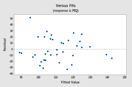
As we scan the plot from left to right, the average of the residuals remains approximately 0, the variation of the residuals appears to be roughly constant, and there are no excessively outlying points (except perhaps the observation with a residual of about 50, which might warrant some further investigation but isn't too much of a worry). Note that the two observations on the right of the plot with fitted values close to 140 are of no concern with respect to the model assumptions. We'd be reading too much into the plot if we were to worry that the residuals appear less variable on the right side of the plot (there are only 2 out of a total of 38 points here and hence there is little information on residual variability in this region of the plot).
- There is no time (or space) variable in this dataset so the next plot we'll consider is a scatterplot with the residuals, \(e_i\), on the vertical axis and one of the predictors in the model, Brain, on the horizontal axis:
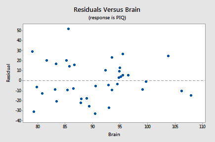
Again, as we scan the plot from left to right, the average of the residuals remains approximately 0, the variation of the residuals appears to be roughly constant, and there are no excessively outlying points. Also, there is no strong nonlinear trend in this plot that might suggest a transformation of PIQ or Brain in this model.
- The next plot we'll consider is a scatterplot with the residuals, \(e_i\), on the vertical axis and the other predictor in the model, Height, on the horizontal axis:
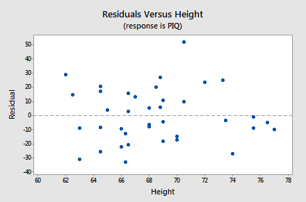
Again, as we scan the plot from left to right, the average of the residuals remains approximately 0, the variation of the residuals appears to be roughly constant, and there are no excessively outlying points. Also, there is no strong nonlinear trend in this plot that might suggest a transformation of PIQ or Height in this model.
- The next plot we'll consider is a histogram of the residuals:
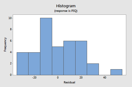
Although this doesn't have the ideal bell-shaped appearance, given the small sample size there's little to suggest a violation of the normality assumption.
- Since the appearance of a histogram can be strongly influenced by the choice of intervals for the bars, to confirm this we can also look at a normal probability plot of the residuals:
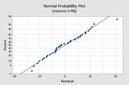
Again, given the small sample size, there's little to suggest a violation of the normality assumption.
- The final plot we'll consider for this example is a scatterplot with the residuals, \(e_i\), on the vertical axis and the only predictor excluded from the model, Weight, on the horizontal axis:
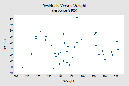
Since there is no strong linear or simple nonlinear trend in this plot, there is nothing to suggest that Weight might be usefully added to the model. Don't get carried away by the apparent "up-down-up-down-up" pattern in this plot. This "trend" isn't nearly strong enough to warrant adding some complex function of Weight to the model - remember we've only got a sample size of 38 and we'd have to use up at least 5 degrees of freedom trying to add a fifth-degree polynomial of Weight to the model. All we'd end up doing if we did this is over-fitting the sample data and ending up with an over-complicated model that predicts new observations very poorly.
One key idea to draw from this example is that if you stare at a scatterplot of completely random points long enough you'll start to see patterns even when there are none! Residual analysis should be done thoroughly and carefully but without over-interpreting every slight anomaly. Serious problems with the multiple linear regression model generally reveal themselves pretty clearly in one or more residual plots. If a residual plot looks "mostly OK," chances are it is fine.
7.5 - Tests for Error Normality
7.5 - Tests for Error NormalityTo complement the graphical methods just considered for assessing residual normality, we can perform a hypothesis test in which the null hypothesis is that the errors have a normal distribution. A large p-value and hence failure to reject this null hypothesis is a good result. It means that it is reasonable to assume that the errors have a normal distribution. Typically, assessment of the appropriate residual plots is sufficient to diagnose deviations from normality. However, a more rigorous and formal quantification of normality may be requested. So this section provides a discussion of some common testing procedures (of which there are many) for normality. For each test discussed below, the formal hypothesis test is written as:
\(\begin{align*} \nonumber H_{0}&\colon \textrm{the errors follow a normal distribution} \\ \nonumber H_{A}&\colon \textrm{the errors do not follow a normal distribution}. \end{align*}\)
While hypothesis tests are usually constructed to reject the null hypothesis, this is a case where we actually hope we fail to reject the null hypothesis as this would mean that the errors follow a normal distribution.
Anderson-Darling Test
The Anderson-Darling Test measures the area between a fitted line (based on the chosen distribution) and a nonparametric step function (based on the plot points). The statistic is a squared distance that is weighted more heavily in the tails of the distribution. Smaller Anderson-Darling values indicate that the distribution fits the data better. The test statistic is given by:
\(\begin{equation*} A^{2}=-n-\sum_{i=1}^{n}\frac{2i-1}{n}(\log \textrm{F}(e_{i})+\log (1-\textrm{F}(e_{n+1-i}))), \end{equation*}\)
where \(\textrm{F}(\cdot)\) is the cumulative distribution of the normal distribution. The test statistic is compared against the critical values from a normal distribution in order to determine the p-value.
The Anderson-Darling test is available in some statistical software. To illustrate here's statistical software output for the example on IQ and physical characteristics from Lesson 5 (IQ Size data), where we've fit a model with PIQ as the response and Brain and Height as the predictors:
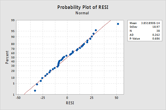
Since the Anderson-Darling test statistic is 0.262 with an associated p-value of 0.686, we fail to reject the null hypothesis and conclude that it is reasonable to assume that the errors have a normal distribution
Shapiro-Wilk Test
The Shapiro-Wilk Test uses the test statistic
\(\begin{equation*} W=\dfrac{\biggl(\sum_{i=1}^{n}a_{i}e_{(i)}\biggr)^{2}}{\sum_{i=1}^{n}(e_{i}-\bar{e})^{2}}, \end{equation*} \)
where \(e_{i}\) pertains to the \(i^{th}\) largest value of the error terms and the \(a_i\) values are calculated using the means, variances, and covariances of the \(e_{i}\). W is compared against tabulated values of this statistic's distribution. Small values of W will lead to the rejection of the null hypothesis.
The Shapiro-Wilk test is available in some statistical software. For the IQ and physical characteristics model with PIQ as the response and Brain and Height as the predictors, the value of the test statistic is 0.976 with an associated p-value of 0.576, which leads to the same conclusion as for the Anderson-Darling test.
Ryan-Joiner Test
The Ryan-Joiner Test is a simpler alternative to the Shapiro-Wilk test. The test statistic is actually a correlation coefficient calculated by
\(\begin{equation*} R_{p}=\dfrac{\sum_{i=1}^{n}e_{(i)}z_{(i)}}{\sqrt{s^{2}(n-1)\sum_{i=1}^{n}z_{(i)}^2}}, \end{equation*}\)
where the \(z_{(i)}\) values are the z-score values (i.e., normal values) of the corresponding \(e_{(i)}\) value and \(s^{2}\) is the sample variance. Values of \(R_{p}\) closer to 1 indicate that the errors are normally distributed.
The Ryan-Joiner test is available in some statistical software. For the IQ and physical characteristics model with PIQ as the response and Brain and Height as the predictors, the value of the test statistic is 0.988 with an associated p-value > 0.1, which leads to the same conclusion as for the Anderson-Darling test.
Kolmogorov-Smirnov Test
The Kolmogorov-Smirnov Test (also known as the Lilliefors Test) compares the empirical cumulative distribution function of sample data with the distribution expected if the data were normal. If this observed difference is sufficiently large, the test will reject the null hypothesis of population normality. The test statistic is given by:
\(\begin{equation*} D=\max(D^{+},D^{-}), \end{equation*}\)
where
\(\begin{align*} D^{+}&=\max_{i}(i/n-\textrm{F}(e_{(i)}))\\ D^{-}&=\max_{i}(\textrm{F}(e_{(i)})-(i-1)/n), \end{align*}\)
The test statistic is compared against the critical values from a normal distribution in order to determine the p-value.
The Kolmogorov-Smirnov test is available in some statistical software. For the IQ and physical characteristics model with PIQ as the response and Brain and Height as the predictors, the value of the test statistic is 0.097 with an associated p-value of 0.490, which leads to the same conclusion as for the Anderson-Darling test.
7.6 - Tests for Constant Error Variance
7.6 - Tests for Constant Error VarianceThere are various tests that may be performed on the residuals for testing if the regression errors have constant variance. It is usually sufficient to "visually" interpret residuals versus fitted values plots. However, the tests we discuss can provide an added layer of justification to your analysis. Note that some of the following procedures require you to partition the residuals into a certain number of groups, say \(g\geq 2\) groups of sizes \(n_{1},\ldots,n_{g}\) such that \(\sum_{i=1}^{g}n_{i}=n\). For these procedures, the sample variance of group i is given by:
\(\begin{equation*} s_{i}^{2}=\dfrac{\sum_{j=1}^{n_{i}}(e_{i,j}-\bar{e}_{i,\cdot})^{2}}{n_{i}-1} \end{equation*} \)
where \(e_{i,j}\) is the \(j^{\textrm{th}}\) residual from group i. Moreover, the pooled variance is given by:
\(\begin{equation*} s_{p}^{2}=\dfrac{\sum_{i=1}^{g}(n_{i}-1)s_{i}^{2}}{n-g} \end{equation*}\)
F-Test
Suppose we partition the residuals of observations into two groups - one consisting of residuals associated with the lowest predictor values and the other consisting of those belonging to the highest predictor values. Treating these two groups as if they could (potentially) represent two different populations, we can test
\(\begin{align*} \nonumber H_{0}&\colon \sigma_{1}^{2}=\sigma_{2}^{2} \\ \nonumber H_{A}&\colon \sigma_{1}^{2}\neq\sigma_{2}^{2} \end{align*}\)
using the F-statistic \(F^{*}=s_{1}^{2}/s_{2}^{2}\). This test statistic is distributed according to a \(F_{n_{1}-1,n_{2}-1}\) distribution, so if \(F^{*}\geq F_{n_{1}-1,n_{2}-1;1-\alpha}\), then reject the null hypothesis and conclude that there is statistically significant evidence that the variance is not constant.
Modified Levene Test
Another test for nonconstant variance is the modified Levene test (sometimes called the Brown-Forsythe test). This test does not require the error terms to be drawn from a normal distribution and hence it is a nonparametric test. The test is constructed by grouping the residuals into g groups according to the values of the quantity on the horizontal axis of the residual plot. It is typically recommended that each group has at least 25 observations and usually g=2 groups are used.
Begin by letting group 1 consist of the residuals associated with the \(n_{1}\) lowest values of the predictor. Then, let group 2 consists of the residuals associated with the \(n_{2}\) highest values of the predictor (so \(n_{1}+n_{2}=n\)). The objective is to perform the following hypothesis test:
\(\begin{align*} \nonumber H_{0}&\colon \textrm{the variance is constant} \\ \nonumber H_{A}&\colon \textrm{the variance is not constant} \end{align*}\)
As with the normality tests considered in the previous section, we hope we fail to reject the null hypothesis as this would mean the variance is constant. The test statistic for the above is computed as follows:
- \(d_{i,j}=|e_{i,j}-\tilde{e}_{i,\cdot}|\), where \(\tilde{e}_{i,\cdot}\) is the median of the \(i^{\textrm{th}}\) group of residuals
- \(s_{L}=\sqrt{\dfrac{\sum_{j=1}^{n_{1}}(d_{1,j}-\bar{d}_{1})^{2}+\sum_{j=1}^{n_{2}}(d_{2,j}-\bar{d}_{2})^{2}}{n_{1}+n_{2}-2}}\)
- \(L=\dfrac{\bar{d}_{1}-\bar{d}_{2}}{s_{L}\sqrt{\frac{1}{n_{1}}+\frac{1}{n_{2}}}}\)
L is approximately distributed according to a \(t_{n_{1}+n_{2}-2}\) distribution, or (equivalently) \(L^2\) is approximately distributed according to an \(F_{1,n_{1}+n_{2}-2}\) distribution.
To illustrate consider the Toluca Company dataset described on page 19 of Applied Linear Regression Models (4th ed) by Kutner, Nachtsheim, and Neter. We fit a simple linear regression model with predictor variable LotSize (the number of refrigerator parts in a production run) and response variable WorkHours (labor hours required to produce a lot of refrigerator parts). A modified Levene test applied with the 13 smallest lot sizes in the first group and the remaining 12 lot sizes in the second group results in the following:
- \(\tilde{e}_1=-19.87596\) and \(\tilde{e}_2=-2.68404\)
- \(\bar{d}_1=44.81507\) and \(\bar{d}_2=28.45034\)
- \(\sum{(d_1-\bar{d}_1)^2}=12566.61\) and \(\sum{(d_2-\bar{d}_2)^2}=9610.287\)
- \(s_L = \sqrt{(12566.61+9610.287)/23} = 31.05178\)
- \(L = (44.81507-28.40534)/(31.05178\sqrt{(1/13+1/12)}) = 1.31648\) and \(L^2=1.7331\)
- The \(t_{23}\) probability area to the left of 1.31648 is 0.8995, which means the p-value for the test is \(2(1-0.8995) = 0.201\), i.e., there is no evidence the errors have nonconstant variance.
Breusch-Pagan Test
The Breusch-Pagan test (also known as the Cook-Weisberg score test) is an alternative to the modified Levene test. Whereas the modified Levene test is a nonparametric test, the Breusch-Pagan test assumes that the error terms are normally distributed, with \(\mbox{E}(\epsilon_{i})=0\) and \(\mbox{Var}(\epsilon_{i})=\sigma^{2}_{i}\) (i.e., nonconstant variance). The \(\sigma_{i}^{2}\) values depend on the horizontal axis quantity (\(X_{i}\)) values in the following way:
\(\begin{equation*} \log\sigma_{i}^{2}=\gamma_{0}+\gamma_{1}X_{i} \end{equation*}\)
We are interested in testing the null hypothesis of constant variance versus the alternative hypothesis of nonconstant variance. Specifically, the hypothesis test is formulated as:
\(\begin{align*} \nonumber H_{0}&\colon \gamma_{1}=0 \\ \nonumber H_{A}&\colon \gamma_{1}\neq 0 \end{align*}\)
This test is carried out by first regressing the squared residuals on the predictor (i.e., regressing \(e_{i}^2\) on \(X_{i}\)). The sum of squares resulting from this analysis is denoted by \(\textrm{SSR}^{*}\), which provides a measure of the dependency of the error term on the predictor. The test statistic is given by:
\(\begin{equation*} X^{2*}=\dfrac{\textrm{SSR}^{*}/2}{(\textrm{SSE}/n)^{2}} \end{equation*}\)
where SSE is from the regression analysis of the response on the predictor. The p-value for this test is found using a \(\chi^{2}\) distribution with 1 degree of freedom (written as \(\chi^{2}_{1}\)).
To illustrate consider the Toluca Company example from above:
- \(SSE=54825\)
- \(SSR^*=7896142\)
- \(X^{2*} = (7896142/2) / (54825/25)^2 = 0.8209\)
- The \(\chi^{2}_{1}\) probability area to the left of 0.8209 is 0.635, which means the p-value for the test is \(1-0.635 = 0.365\), i.e., there is no evidence the errors have nonconstant variance.
When the variance is a function of q > 1 predictor, SSR* derives from a multiple regression of the squared residuals against these predictors, and there are q degrees of freedom for the \(\chi^{2}\) distribution.
Bartlett's Test
Bartlett's test is another test that can be used to test for constant variance. The objective is to again perform the following hypothesis test:
\(\begin{align*}\nonumber H_{0}\colon \textrm{the variance is constant} \\ \nonumber H_{A}\colon \textrm{the variance is not constant}\end{align*} \)
Bartlett's test is highly sensitive to the normality assumption, so if the residuals do not appear normal (even after transformations), then this test should not be used. Instead, the Levene test is the alternative to Bartlett's test which is less sensitive to departures from normality.
This test is carried out similarly to the Levene test. Once you have partitioned the residuals into g groups, the following test statistic can be constructed:
\(\begin{equation*} B=\dfrac{(n-g)\ln s_{p}^{2}-\sum_{i=1}^{g}(n_{i}-1)\ln s_{i}^{2}}{1+\biggl(\dfrac{1}{3(g-1)}\biggl((\sum_{i=1}^{g}\dfrac{1}{n_{i}-1})-\dfrac{1}{n-g}\biggr)\biggr)} \end{equation*}\)
The test statistic B is distributed according to a \(\chi^{2}_{g-1}\) distribution, so if \(B\geq \chi^{2}_{g-1;1-\alpha}\), then reject the null hypothesis and conclude that there is statistically significant evidence that the variance is not constant.
7.7 - Data Transformations
7.7 - Data TransformationsData transformations are used in regression to describe curvature and can sometimes be usefully employed to correct for violation of the assumptions in a multiple linear regression model (particularly the "L" and "E" assumptions). We'll return to this topic in more detail in Lesson 9.
Software Help 7
Software Help 7The next two pages cover the Minitab and commands for the procedures in this lesson.
Below is a text file that contains the data used in this lesson:
Minitab Help 7: MLR Estimation, Prediction & Model Assumptions
Minitab Help 7: MLR Estimation, Prediction & Model AssumptionsMinitab®
IQ and physical characteristics (confidence and prediction intervals)
- Perform a linear regression analysis of PIQ on Brain and Height.
- Find a confidence interval and a prediction interval for the response.
IQ and physical characteristics (residual plots and normality tests)
- Perform a linear regression analysis of PIQ on Brain and Height.
- Create residual plots and select "Residuals versus fits" (with regular residuals).
- Create residual plots and specify Brain, Height, and Weight in the "Residuals versus the variables" box (with regular residuals).
- Create residual plots and select "Histogram of residuals" (with regular residuals).
- Create residual plots and select "Normal probability plot of residuals" (with regular residuals).
- Conduct regression error normality tests and select:
- Anderson-Darling
- Ryan-Joiner (similar to Shapiro-Wilk)
- Kolmogorov-Smirnov (Lilliefors)
Toluca refrigerator parts (tests for constant error variance)
- Perform a linear regression analysis of WorkHours on LotSize and store the residuals, RESI.
- Modified Levene (Brown-Forsythe):
- Select Data > Code > To Text, select LotSize for "Code values in the following columns," select "Code ranges of values" for "Method," type "20" for the first lower endpoint, type "70" for the first upper endpoint, type "1" for the first coded value, type "80" for the second lower endpoint, type "120" for the second upper endpoint, type "2" for the second coded value, select "Both endpoints" for "Endpoints to include," and click OK.
- Select Stat > Basic Statistics > Store Descriptive Statistics, select RESI for "Variables," select 'Coded LotSize' for "By variables," click "Statistics," select "Median," and click OK. This calculates \(\tilde{e}_1=-19.876\) and \(\tilde{e}_2=-2.684\).
- Select Calc >Calculator, type "d" for "Store result in variable," type "abs('RESI'-IF('Coded LotSize'="1",-19.876,-2.684))" for "Expression," and click OK. This calculates d1 and d2.
- Select Stat > Basic Statistics > Store Descriptive Statistics, select d for "Variables," select 'Coded LotSize' for "By variables," click "Statistics," select "Mean," and click OK. This calculates \(\bar{d}_1=44.8151\) and \(\bar{d}_2=28.4503\).
- Select Calc >Calculator, type "devsq" for "Store result in variable," type "(d-IF('Coded LotSize'="1",44.8151,28.4503))^2" for "Expression," and click OK. This calculates \((d_1-\bar{d}_1)^2\) and \((d_2-\bar{d}_2)^2\).
- Select Stat > Basic Statistics > Store Descriptive Statistics, select devsq for "Variables," select 'Coded LotSize' for "By variables," click "Statistics," select "Sum," and click OK. This calculates \(\sum{(d_1-\bar{d}_1)^2}=12566.6\) and \(\sum{(d_2-\bar{d}_2)^2}=9610.3\).
- We can then calculate \(s_L = \sqrt{(12566.6+9610.3)/23} = 31.05\) and \(L = (44.8151-28.4053)/(31.05\sqrt{(1/13+1/12)}) = 1.316\).
- Select Calc > Probability Distributions > t, type "23" for "Degrees of freedom," select "Input constant," type "1.316," and click OK. This calculates the probability area to the left of 1.316 as 0.89943, which means the p-value for the test is \(2(1-0.89943) = 0.20\), i.e., there is no evidence the errors have nonconstant variance.
- Breusch-Pagan (Cook-Weisberg score):
- Select Calc >Calculator, type "esq" for "Store result in variable," type "'RESI'^2" for "Expression," and click OK. This calculates the squared residuals.
- Fit the model with response esq and predictor LotSize. Observe SSR* = 7896142.
- We can then calculate \(X^{2*} = (7896142/2) / (54825/25)^2 = 0.821\).
- Select Calc > Probability Distributions > Chi-Square, type "1" for "Degrees of freedom," select "Input constant," type "0.821," and click OK. This calculates the probability area to the left of 0.821 as 0.635112, which means the p-value for the test is \(1-0.635112 = 0.36\), i.e., there is no evidence the errors have nonconstant variance.
R Help 7: MLR Estimation, Prediction & Model Assumptions
R Help 7: MLR Estimation, Prediction & Model AssumptionsR Help
IQ and physical characteristics (confidence and prediction intervals)
- Load the iqsize data.
- Fit a multiple linear regression model of PIQ on Brain and Height.
- Calculate a 95% confidence interval for mean PIQ at Brain=90, Height=70.
- Calculate a 95% confidence interval for mean PIQ at Brain=79, Height=62.
- Calculate a 95% prediction interval for individual PIQ at Brain=90, Height=70.
iqsize <- read.table("~/path-to-folder/iqsize.txt", header=T)
attach(iqsize)

predict(model, interval="confidence", se.fit=T,
        newdata=data.frame(Brain=90, Height=70))
# $fit
#        fit      lwr     upr
# 1 105.6391 98.23722 113.041
#
# $se.fit
# [1] 3.646064

predict(model, interval="confidence", se.fit=T,
        newdata=data.frame(Brain=79, Height=62))
# $fit
#        fit      lwr     upr
# 1 104.8114 91.41796 118.2049
#
# $se.fit
# [1] 6.597407

predict(model, interval="prediction",
        newdata=data.frame(Brain=90, Height=70))
# $fit
#        fit      lwr     upr
# 1 105.6391 65.34688 145.9314

detach(iqsize)
IQ and physical characteristics (residual plots and normality tests)
- Load the iqsize data.
- Fit a multiple linear regression model of PIQ on Brain and Height.
- Display the residual plot with fitted (predicted) values on the horizontal axis.
- Display the residual plot with Brain on the horizontal axis.
- Display the residual plot with Height on the horizontal axis.
- Display the histogram of the residuals.
- Display a normal probability plot of the residuals and add a diagonal line to the plot. The argument "datax" determines which way round to plot the axes (false by default, which plots the data on the vertical axis, or true, which plots the data on the horizontal axis).
- Display residual plot with Weight on the horizontal axis.
- Load the
nortestpackage to access normality tests:- Anderson-Darling
- Shapiro-Wilk (Ryan-Joiner unavailable in R)
- Lilliefors (Kolmogorov-Smirnov)
iqsize <- read.table("~/path-to-folder/iqsize.txt", header=T)
attach(iqsize)

model <- lm(PIQ ~ Brain + Height)

plot(x=fitted(model), y=residuals(model),
     xlab="Fitted values", ylab="Residuals",
     panel.last = abline(h=0, lty=2))

plot(x=Brain, y=residuals(model),
     ylab="Residuals",
     panel.last = abline(h=0, lty=2))

plot(x=Height, y=residuals(model),
     ylab="Residuals",
     panel.last = abline(h=0, lty=2))

hist(residuals(model), main="")

qqnorm(residuals(model), main="", datax=TRUE)
qqline(residuals(model), datax=TRUE)

plot(x=Weight, y=residuals(model),
     ylab="Residuals",
     panel.last = abline(h=0, lty=2))

library(nortest)
ad.test(residuals(model)) # A = 0.2621, p-value = 0.6857
shapiro.test(residuals(model)) # W = 0.976, p-value = 0.5764
lillie.test(residuals(model)) # D = 0.097, p-value = 0.4897

detach(iqsize)
Toluca refrigerator parts (tests for constant error variance)
- Load the Toluca data.
- Fit a simple linear regression model of WorkHours on LotSize.
- Create lotgroup factor variable splitting the sample into two groups.
- Load the
carpackage to access tests for constant error variance:- Modified Levene (Brown-Forsythe)
- Cook-Weisberg score (Breusch-Pagan)
toluca <- read.table("~/path-to-folder/toluca.txt", header=T)
attach(toluca)

model <- lm(WorkHours ~ LotSize)
lotgroup <- factor(LotSize<=70)

library(car)
leveneTest(residuals(model), group=lotgroup)
# Levene's Test for Homogeneity of Variance (center = median)
#       Df F value Pr(>F)
# group  1  1.7331  0.201
#       23

ncvTest(model)
# Non-constant Variance Score Test
# Variance formula: ~ fitted.values
# Chisquare = 0.8209192    Df = 1     p = 0.3649116

detach(toluca)