Lesson 8: Categorical Predictors
Lesson 8: Categorical PredictorsOverview
In Lesson 6, we utilized a multiple regression model that contained binary or indicator variables to code the information about the treatment group to which rabbits had been assigned. In this lesson, we investigate the use of such indicator variables for coding qualitative or categorical predictors in multiple linear regression more extensively. Although we primarily focus on categorical predictors with just two categories or levels, the methods and concepts extend readily to general categorical variables that, rather than defining just two groups, define c groups.
What happens if the effect of a categorical predictor on the response y depends on another (quantitative) predictor? In that case, we say that the predictors "interact." In this lesson, we learn how to formulate multiple regression models that contain "interaction effects" as a way to account for predictors that do interact.
We also investigate a special kind of model—called a "piecewise linear regression model"—that uses an interaction term as a way of creating a model that contains two or more different linear pieces.
Objectives
- Formulate a multiple regression model that contains one qualitative (categorical) predictor and one quantitative predictor.
- Determine the different mean response functions for different levels of a qualitative (categorical) predictor variable.
- Answer certain research questions based on a regression model with one qualitative (categorical) predictor and one quantitative predictor.
- Understand and appreciate the two advantages of fitting one regression function rather than separate regression functions — one for each level of the qualitative (categorical) predictor
- Properly code a qualitative variable so that it can be incorporated into a multiple regression model.
- Be able to figure out the impact of using different coding schemes.
- Interpret the regression coefficients of a linear regression model containing a qualitative (categorical) predictor variable.
- Understand the distinction between additive effects and interaction effects.
- Understand the impact of including an interaction term in a regression model.
- Know how to use a formulated model to determine how to test whether there is an interaction between a qualitative (categorical) predictor and a quantitative predictor.
- Know how to answer various research questions for models with interaction terms.
- Know the impact of leaving a necessary interaction term out of the model.
- Know how to formulate a piecewise linear regression model for two or more connected linear pieces.
Lesson 8 Code Files
Below is a zip file that contains all the data sets used in this lesson:
- birthsmokers.txt
- birthsmokers_02.txt
- depression.txt
- leadmoss.txt
- shipment
8.1 - Example on Birth Weight and Smoking
8.1 - Example on Birth Weight and SmokingExample 8-1: Birth weight and Smoking during pregnancy

Researchers (Daniel, 1999) interested in answering the above research question collected the following data (Birth and Smokers dataset) on a random sample of n = 32 births:
- Response (y): birth weight (Weight) in grams of baby
- Potential predictor \(\left(x_{1}\right)\colon\) Smoking status of mother (yes or no)
- Potential predictor \(\left(x_{2}\right)\colon\) length of gestation (Gest) in weeks
The distinguishing feature of this data set is that one of the predictor variables — Smoking — is a qualitative predictor. To be more precise, smoking is a "binary variable" with only two possible values (yes or no). The other predictor variable (Gest) is, of course, quantitative.
The scatter plot matrix:
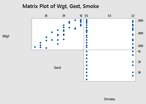
suggests, not surprisingly, that there is a positive linear relationship between the length of gestation and birth weight. That is, as the length of gestation increases, the birth weight of babies tends to increase. It is hard to see if any kind of (marginal) relationship exists between birth weight and smoking status, or between the length of gestation and smoking status.
The important question remains — after taking into account the length of gestation, is there a significant difference in the average birth weights of babies born to smoking and non-smoking mothers? A first-order model with one binary predictor and one quantitative predictor that helps us answer the question is:
\(y_i=(\beta_0+\beta_1x_{i1}+\beta_2x_{i2})+\epsilon_i\)
where:
- \(y_{i}\) is the birth weight of baby i
- \(x_{i1}\) is the length of gestation of baby i
- \(x_{i2}\) is a binary variable coded as a 1 if the baby's mother smoked during pregnancy and 0 if she did not
and the independent error terms \(\epsilon_i\) follow a normal distribution with mean 0 and equal variance \(\sigma^{2}\).
Notice that to include a qualitative variable in a regression model, we have to "code" the variable, that is, assign a unique number to each of the possible categories. We'll learn more about coding in the remainder of this lesson.
Using the sample data on n = 32 births, the plot of the estimated regression function looks like this:
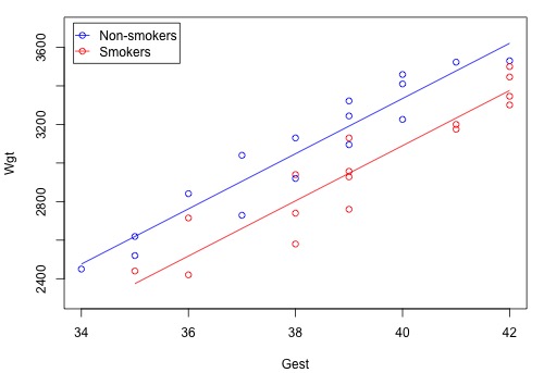
The blue circles represent the data on non-smoking mothers \(\left(x_2 = 0 \right) \), while the red circles represent the data on smoking mothers \(\left(x_{2} = 1\right)\). And, the blue line represents the estimated linear relationship between the length of gestation and birth weight for non-smoking mothers, while the red line represents the estimated linear relationship for smoking mothers.
At least in this sample of data, it appears as if the birth weights for non-smoking mothers are higher than that for smoking mothers, regardless of the length of gestation. A hypothesis test or confidence interval would allow us to see if this result extends to the larger population.
Did you expect the plot of the estimated regression equation to appear as two distinct lines? Let's consider this question. Minitab tells us that the estimated regression function is:
Regression Equation
Wgt = - 2390 + 143.10 Gest - 244.5 Smoke
Therefore, as illustrated in this screencast below, the estimated regression equation for non-smoking mothers (smoking = 0) is:
\(\widehat{Weight} = - 2390 + 143 Gest\)
and the estimated regression equation for smoking mothers (when smoking = 1) is:
\(\widehat{Weight} = - 2635 + 143 Gest\)
That is, we obtain two different parallel estimated lines (they are parallel because they have the same slope, 143). The difference between the two lines, –245, represents the difference in the average birth weights for a fixed gestation length for smoking and non-smoking mothers in the sample.
How would we answer the following set of research questions? (Do the procedures that appear in parentheses seem appropriate in answering the research question?)
- Is the baby's birth weight related to smoking during pregnancy, after taking into account the length of gestation? (Conduct a hypothesis test for testing whether the slope parameter for smoking is 0.)
- How is birth weight related to gestation, after taking into account a mother's smoking status? (Calculate and interpret a confidence interval for the slope parameter for gestation.)
Upon analyzing the data, the Minitab output:
Regression Analysis: Wgt versus Gest, Smoke
Analysis of Variance
| Source | DF | Adj SS | Adj MS | F-Value | P-Value |
|---|---|---|---|---|---|
| Regression | 2 | 3348720 | 1674360 | 125.45 | 0.000 |
| Gest | 1 | 3280270 | 3280270 | 245.76 | 0.000 |
| Smoke | 1 | 452881 | 452881 | 33.93 | 0.000 |
| Error | 29 | 387070 | 13347 | ||
| Lack-of-Fit | 12 | 52383 | 4365 | 0.22 | 0.994 |
| Pure Error | 17 | 334687 | 19687 | ||
| Total | 31 | 3735790 |
Model Summary
| S | R-sq | R-sq(adj) | R-sq(pred) |
|---|---|---|---|
| 115.530 | 89.64% | 88.92% | 87.6% |
Coefficients
| Term | Coef | SE Coef | T-Value | P-Value | VIF |
|---|---|---|---|---|---|
| Constant | -2390 | 349 | -6.84 | 0.000 | |
| Gest | 143.10 | 9.13 | 15.68 | 0.000 | 1.06 |
| Smoke | -244.5 | 42.0 | -5.83 | 0.000 | 1.06 |
Regression Equation
Wgt = - 2390 + 143.10 Gest - 244.5 Smoke
tells us that:
- A whopping 89.64% of the variation in the birth weights of babies is explained by the length of gestation and the smoking status of the mother.
- The P-values for the t-tests appearing in the table of estimates suggest that the slope parameters for Gest (P < 0.001) and Smoking (P < 0.001) are significantly different from 0.
- The P-value for the analysis of variance F-test (P < 0.001) suggests that the model containing the length of gestation and smoking status is more useful in predicting birth weight than not taking into account the two predictors.
8.2 - The Basics
8.2 - The BasicsA "binary predictor" is a variable that takes on only two possible values. Here are a few common examples of binary predictor variables that you are likely to encounter in your own research:
- Gender (male, female)
- Smoking status (smoker, nonsmoker)
- Treatment (yes, no)
- Health status (diseased, healthy)
- Company status (private, public)
Example 8-2: On average, do smoking mothers have babies with lower birth weight?
In the previous section, we briefly investigated data (Birth and Smokers data) on a random sample of n = 32 births that allow researchers (Daniel, 1999) to answer the above research question. The researchers collected the following data:
- Response \(\left(y\right)\colon\) birth weight (Weight) in grams of baby
- Potential predictor \(\left(x_1\right)\colon\) length of gestation (Gest) in weeks
- Potential predictor \(\left(y\right)\colon\) Smoking status of mother (smoker or non-smoker)
To include a qualitative variable in a regression model, we have to "code" the variable, that is, assign a unique number to each of the possible categories. A common coding scheme is to use what's called a "zero-one-indicator variable." Using such a variable here, we code the binary predictor Smoking as:
- \(x_{i2} = 1\), if mother i smokes
- \(x_{i2} = 0\), if mother i does not smoke
In doing so, we use the tradition of assigning the value of 1 to those having the characteristic of interest and 0 to those not having the characteristic. Tradition is less important, though than making sure you keep track of your coding scheme so that you can properly draw conclusions. Incidentally, other terms sometimes used instead of "zero-one-indicator variable" are "dummy variable" or "binary variable".
A scatter plot of the data in which blue circles represent the data on non-smoking mothers \(\left(x_{2} = 0 \right)\) and red circles represent the data on smoking mothers \(\left(x_{2} = 1 \right)\colon \)
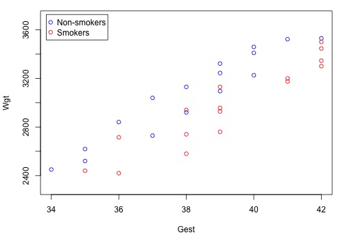
suggests that there might be two distinct linear trends in the data — one for smoking mothers and one for non-smoking mothers. Therefore, a first-order model with one binary and one quantitative predictor appears to be a natural model to formulate for these data. That is:
\(y_i=(\beta_0+\beta_1x_{i1}+\beta_2x_{i2})+\epsilon_i\)
where:
- \(y_{i}\) is the birth weight of baby i in grams
- \(x_{i1}\) is the length of gestation of baby i in weeks
- \(x_{i2} = 1\), if the mother smoked during pregnancy, and \(x_{i2} = 0\), if she did not
and the independent error terms \(\epsilon_{i}\) follow a normal distribution with mean 0 and equal variance \(\sigma^{2}\).
How does a model containing a (0,1) indicator variable for two groups yield two distinct response functions? In short, this screencast below illustrates how the mean response function:
\(\mu_Y=\beta_0+\beta_1x_{i1}+\beta_2x_{i2}\)
yields one regression function for non-smoking mothers \(\left(x_{i2} = 0\right)\colon\)
\(\mu_Y=\beta_0+\beta_1x_{i1}\)
and one regression function for smoking mothers \(\left(x_{i2} = 1\right)\colon\)
\(\mu_Y=(\beta_0+\beta_2)+\beta_1x_{i1}\)
Note that the two formulated regression functions have the same slope \(\left(\beta_1\right)\) but different intercepts \(\left(\beta_0\ \text{and}\ \beta_0 + \beta_2 \right)\) — mathematical characteristics that, based on the above scatter plot, appear to summarize the trend in the data well.
Now, given that we generally use regression models to answer research questions, we need to figure out how each of the parameters in our model enlightens us about our research problem! The fundamental principle is that you can determine the meaning of any regression coefficient by seeing what effect changing the value of the predictor has on the mean response μY. Here's the interpretation of the regression coefficients in a regression model with one (0, 1) binary indicator variable and one quantitative predictor:
- \(\beta_1\) represents the change in the mean response \(\mu_Y\) for each additional unit increase in the quantitative predictor \(x_1\) ... for both groups.
- \(\beta_2\) represents how much higher (or lower) the mean response function of the second group is than that of the first group... for any value of \(x_1\).
Upon fitting our formulated regression model to our data, Minitab tells us:
Regression Equation
Wgt = - 2390 + 143.10 Gest - 244.5 Smoke
Unfortunately, Minitab doesn't precede the phrase "regression equation" with the adjective "estimated" to emphasize that we've only obtained an estimate of the actual unknown population regression function. But anyway — if we set Smoking once equal to 0 and once equal to 1 — we obtain, as hoped, two distinct estimated lines:
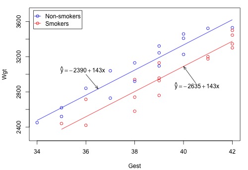
Now, let's use our model and analysis to answer the following research question: Is there a significant difference in mean birth weights for the two groups, after taking into account the length of gestation? As is always the case, the first thing we need to do is to "translate" the research question into an appropriate statistical procedure. We can show that if the slope parameter \(\beta_2\) is 0, there is no difference in the means of the two groups — for any length of gestation. That is, we can answer our research question by testing the null hypothesis \(H_0 \colon \beta_2 = 0\) against the alternative \(H_{A} \colon \beta_2 \ne 0\).
Well, that's easy enough! The Minitab output:
Model Summary
| S | R-sq | R-sq(adj) | R-sq(pred) |
|---|---|---|---|
| 115.530 | 89.64% | 88.92% | 87.60% |
Model Summary
| Term | Coef | SE Coef | T-Value | P-Value | VIF |
|---|---|---|---|---|---|
| Constant | -2390 | 349 | -6.84 | 0.000 | |
| Gest | 143.10 | 9.13 | 15.68 | 0.000 | 1.06 |
| Smoke | -244.5 | 42.0 | -5.83 | 0.000 | 1.06 |
Regression Equation
Wgt = - 2390 + 143.10 Gest - 244.5 Smoke
Reports that the P-value is < 0.001 for testing \(H_0 \colon \beta_2 = 0\). At just about any significance level, we can reject the null hypothesis \(H_0 \colon \beta_2 = 0\) in favor of the alternative hypothesis \(H_{A} \colon \beta_2 \ne 0\). There is sufficient evidence to conclude that there is a statistically significant difference in the mean birth weight of all babies of smoking mothers and the mean birth weight of babies of all non-smoking mothers, after taking into account the length of gestation.
A 95% confidence interval for \(\beta_2\) tells us the magnitude of the difference. A 95% t-multiplier with n-p = 32-3 = 29 degrees of freedom is \(t_{\left(0.025, 29\right)} = 2.0452\). Therefore, a 95% confidence interval for \(\beta_2\) is:
-244.54 ± 2.0452(41.98) or (-330.4, -158.7).
We can be 95% confident that the mean birth weight of smoking mothers is between 158.7 and 330.4 grams less than the mean birth weight of non-smoking mothers, regardless of the length of gestation. It is up to the researchers to debate whether or not the difference is meaningful.
Try it!
A model with a binary predictor
\(\mu_Y|(x_{i1}=x+1) = \beta_0+\beta_1(x+1)\)
\(\mu_Y|(x_{i1}=x) = \beta_0+\beta_1 x\)
Take the difference,
\(\mu_Y|(x_{i1}=x+1) - \mu_Y|(x_{i1}=x) = \beta_0+\beta_1(x+1) - (\beta_0+\beta_1 x) = \beta_1\)
8.3 - Two Separate Advantages
8.3 - Two Separate AdvantagesPerhaps somewhere along the way in our most recent discussion, you thought "why not just fit two separate regression functions — one for the smokers and one for the non-smokers?" (If you didn't think of it, I thought of it for you!) Are there advantages to including both the binary and quantitative predictor variables within one multiple regression model? The answer is yes! In this section, we explore the two primary advantages.
The first advantage
An easy way of discovering the first advantage is to analyze the data three times — once using the data on all 32 subjects, using the data on only the 16 non-smokers, and once using the data on only the 16 smokers. Then, we can investigate the effects of the different analyses on important things such as the sizes of standard errors of the coefficients and the widths of confidence intervals. Let's try it!
Here's the Minitab output for the analysis using a (0,1) indicator variable and the data on all 32 subjects. Let's just run through the output and collect information on various values obtained:
Coefficients
| Term | Coef | SE Coef | T-Value | P-Value | VIF |
|---|---|---|---|---|---|
| Constant | -2390 | 349 | -6.84 | 0.000 | |
| Gest | 143.10 | 9.13 | 15.68 | 0.000 | 1.06 |
| Smoke | -244.5 | 42.0 | -5.83 | 0.000 | 1.06 |
Regression Equation
Wgt = -2390 + 143.10 Gest - 244.5 SmokeThe standard error of the Gest coefficient is 9.13. Recall that this value quantifies how much the estimated Gest coefficient would vary from sample to sample. And, the following output:
Variable Setting
| Gest | 38 |
|---|---|
| Smoke | 1 |
| Fit | SE Fit | 95% CI | 95% PI |
|---|---|---|---|
| 2803.69 | 30.8496 | (2740.60, 2866.79) | (2559.13, 3048.26) |
Variable Setting
| Gest | 38 |
|---|---|
| Smoke | 0 |
| Fit | SE Fit | 95% CI | 95% PI |
|---|---|---|---|
| 3048.24 | 28.9051 | (2989.12, 3107.36) | (2804.67, 3291.81) |
tells us that for mothers with a 38-week gestation, the width of the confidence interval for the mean birth weight is 126.2 for smoking mothers and 118.2 for non-smoking mothers.
Let's do that again, but this time for the Minitab output on just the 16 non-smoking mothers:
Coefficients
| Term | Coef | SE Coef | T-Value | P-Value | VIF |
|---|---|---|---|---|---|
| Constant | -2546 | 457 | -5.57 | 0.000 | |
| Gest_0 | 147.2 | 12.0 | 12.29 | 0.000 | 1.00 |
Regression Equation
Wgt_0 = -2546 + 147.2 Gest_0The standard error of the Gest coefficient is 12.0. And:
| Variable | Setting |
|---|---|
| Gest_0 | 38 |
| Fit | SE Fit | 95% CI | 95% PI |
|---|---|---|---|
| 3047.72 | 26.7748 | (2990.30, 3105.15) | (2811.30, 3284.15) |
for non-smoking mothers with a 38-week gestation, the width of the confidence interval for the mean birth weight is 114.9.
And, let's do the same thing one more time for the Minitab output on just the 16 smoking mothers:
Coefficients
| Term | Coef | SE Coef | T-Value | P-Value | VIF |
|---|---|---|---|---|---|
| Constant | -2475 | 554 | -4.447 | 0.001 | |
| Gest_1 | 139.0 | 14.1 | 9.85 | 0.000 | 1.00 |
Regression Equation
Wgt_1 = -2475 + 139.2 Gest_1The standard error of the Gest coefficient is 14.1. And:
| Variable | Setting |
|---|---|
| Gest_1 | 38 |
| Fit | SE Fit | 95% CI | 95% PI |
|---|---|---|---|
| 2808.53 | 35.8088 | (2731.73, 2885.33) | (2526.39, 3090.67) |
for smoking mothers with a 38-week gestation, the length of the confidence interval is 153.6.
Here's a summary of what we've gleaned from the three pieces of output:
| Model estimated using… |
SE(Gest)
|
Width of CI for \(\mu_Y\) |
|---|---|---|
| all 32 data points |
9.13
|
(NS) 118.2
(S) 126.2 |
| 16 nonsmokers |
12.0
|
114.9
|
| 16 smokers |
14.1
|
153.6
|
Let's see what we learn from this investigation:
- The standard error of the Gest coefficient — SE(Gest) — is the smallest for the estimated model based on all 32 data points. Therefore, confidence intervals for the Gest coefficient will be narrower if calculated using the analysis based on all 32 data points. (This is a good thing!)
- The width of the confidence interval for the mean weight of babies born to smoking mothers is narrower for the estimated model based on all 32 data points (126.2 compared to 153.6), and not substantially different for non-smoking mothers (118.2 compared to 114.9). (Another good thing!)
In short, there appears to be an advantage in "pooling" and analyzing the data all at once rather than breaking it apart and conducting different analyses for each group. Our regression model assumes that the slope for the two groups is equal. It also assumes that the variances of the error terms are equal. Therefore, it makes sense to use as much data as possible to estimate these quantities.
The second advantage
An easy way of discovering the second advantage of fitting one "combined" regression function using all of the data is to consider how you'd answer the research question if you broke apart the data and conducted two separate analyses obtaining:
Nonsmokers
Coefficients
| Term | Coef | SE Coef | T-Value | P-Value | VIF |
|---|---|---|---|---|---|
| Constant | -2546 | 457 | -5.57 | 0.000 | |
| Gest_0 | 147.2 | 12.0 | 12.29 | 0.000 | 1.00 |
Regression Equation
Wgt_0 = -2546 + 147.2 Gest_0Smokers
Coefficients
| Term | Coef | SE Coef | T-Value | P-Value | VIF |
|---|---|---|---|---|---|
| Constant | -2475 | 554 | -4.47 | 0.001 | |
| Gest_1 | 139.0 | 14.1 | 9.85 | 0.000 | 1.00 |
Regression Equation
Wgt_1 = -2475 + 139.0 Gest_1How could you use these results to determine if the mean birth weight of babies differs between smoking and non-smoking mothers, after taking into account the length of gestation? Not completely obvious is it?! It actually could be done with much more (complicated) work than would be necessary if you analyze the data as a whole and fit one combined regression function:
Coefficients
| Term | Coef | SE Coef | T-Value | P-Value | VIF |
|---|---|---|---|---|---|
| Constant | -2390 | 349 | -6.84 | 0.000 | |
| Gest | 143.10 | 9.13 | 15.68 | 0.000 | 1.06 |
| Smoke | -244.5 | 42.0 | -5.83 | 0.000 | 1.06 |
Regression Equation
Wgt = -2390 + 143.10 Gest - 244.5 SmokeAs we previously discussed, answering the research question merely involves testing the null hypothesis \(H_0 \colon \beta_2 = 0\) against the alternative \(H_0 \colon \beta_2 \ne 0\). The P-value is < 0.001. There is sufficient evidence to conclude that there is a statistically significant difference in the mean birth weight of all babies of smoking mothers and the mean birth weight of all babies of non-smoking mothers, after taking into account the length of gestation.
In summary, "pooling" your data and fitting one combined regression function allows you to easily and efficiently answer research questions concerning the binary predictor variable.
8.4 - Coding Qualitative Variables
8.4 - Coding Qualitative VariablesIn this section, we focus on issues concerning the coding of qualitative variables. In particular, we:
- learn a general rule for the number of indicator variables that are necessary for coding a qualitative variable
- investigate the impact of using a different coding scheme, such as (1, -1) coding, on the interpretation of the regression coefficients
A general rule for coding a qualitative variable
In the birth weight example, we coded the qualitative variable Smoking by creating a (0, 1) indicator variable that took on the value 1 for smoking mothers and 0 for non-smoking mothers. What if we had instead tried to use two indicator variables? That is, what if we created one (0, 1) indicator variable, \(x_{i2}\) say, for smoking mothers defined as:
- \(x_{i2} = 1\), if mother smokes
- \(x_{i2} = 0\), if mother does not smoke
and one (0, 1) indicator variable, \(x_{i3}\) say, for non-smoking mothers defined as:
- \(x_{i3} = 1\), if mother does not smoke
- \(x_{i3} = 0\), if mother smokes
In this case, our modified regression function with two binary predictors and one quantitative predictor would be:
\(\mu_Y=\beta_0+\beta_1x_{i1}+\beta_2x_{i2}+\beta_3x_{i3}\)
where:
- \(\mu_{Y}\) is the mean birth weight for given predictors
- \(x_{i1}\) is the length of gestation of baby i
- \(x_{i2} = 1\), if mother smokes and \(x_{i2} = 0\), if mother does not
- \(x_{i3} = 1\), if mother does not smoke and \(x_{i3} = 0\), if mother smokes
Do you see where this is going? Let's see what the implication of such a coding scheme is on the data analysis:
Regression Analysis: Weight versus gest, x2*, x3*
* x3* is highly correlated with other X variables
* x3* has been removed from the equation
The regression equation is
Weight = -2390 + 143 Gest - 245 x2*
| Predictor | Coef | SE Coef | T | P |
|---|---|---|---|---|
| Constant | -2389.6 | 349.2 | -6.84 | 0.000 |
| Gest | -143.100 | 9.128 | 15.68 | 0.000 |
| x2* | -244.54 | 41.98 | -5.83 | 0.000 |
| Modal Summary | ||
|---|---|---|
| S = 115.5 | R-Sq = 89.6% | R-Sq(adj) = 88.9% |
As you can see in blue, Minitab has problems with fitting the model. This is not a problem unique to Minitab — any statistical software would have problems. At issue is that the indicator variable \(x_{3}\) is "highly correlated" with the indicator variable \(x_{2}\) . In fact, \(x_{2}\) and \(x_{3}\) are perfectly correlated with one another — when \(x_{2}\) is 1, \(x_{3}\) is always 0 and when \(x_{2}\) is 0, \(x_{3}\) is always 1. (Described more technically, the columns of the X matrix are linearly dependent — if you add the \(x_{2}\) and \(x_{3}\) columns you get the column of 1's for the intercept term.) As you can see ("x3 has been removed from the equation"), Minitab attempts to fix the problem for us by dropping from the model the last predictor variable listed.
How do we prevent such problems from occurring when coding a qualitative variable? The short answer is to always create one fewer indicator variable than the number of groups defined by the qualitative variable. That is, in general, a qualitative variable defining c groups should be represented by c - 1 indicator variables, each taking on values 0 and 1. For example:
- If your qualitative variable defines 2 groups, then you need 1 indicator variable.
- If your qualitative variable defines 3 groups, then you need 2 indicator variables.
- If your qualitative variable defines 4 groups, then you need 3 indicator variables.
And, so on.
Then, choose one group or category to be the "reference" group (often it will be clear from the application which group should be the reference group, such as a control group in a medical experiment, but, if not, then the group with the most observations is often a good choice; if all groups are the same size and there is no obvious reference group then simply select the most convenient group). Observations in this group will have the value zero for all the indicator variables used to code this qualitative variable. Each of the remaining c – 1 groups will be represented by one and only one of the c – 1 indicator variables. For examples of how this works in practice, see the three-group examples in Section 6.1, where "no cooling" is the reference group, and Section 8.6, where treatment C is the reference group.
The impact of using a different coding scheme
In the birth weight example, we coded the qualitative variable Smoking by creating a (0, 1) indicator variable that took on the value 1 for smoking mothers and 0 for non-smoking mothers. What if we had instead used (1, -1) coding? That is, what if we created a (1, -1) indicator variable, \(x_{i2}\) say, defined as:
- \(x_{i2} = 1\), if the mother smokes
- \(x_{i2} = -1\), if mother does not smoke
In this case, our modified regression function using a (1, -1) coding scheme would be:
\(y_i=(\beta_0+\beta_1x_{i1}+\beta_2x_{i2})+\epsilon_i\)
where:
- \(y_{i}\) is the birth weight of baby i
- \(x_{i1}\) is the length of gestation of baby i
- \(x_{i2} = 1\), if the mother smokes and \(x_{i2} = -1\), if the mother does not smoke
The mean response function:
\(\mu_Y=\beta_0+\beta_1x_{i1}+\beta_2x_{i2}\)
yields two different response functions. If the mother is a non-smoker, then \(x_{i2} = -1\) and the mean response function looks like:
\(\mu_Y=(\beta_0-\beta_2)+\beta_1x_{i1}\)
while if the mother is a smoker, then \(x_{i2} = 1\) and the mean response function looks like this:
\(\mu_Y=(\beta_0+\beta_2)+\beta_1x_{i1}\)
Recall that the fundamental principle is that you can determine the meaning of any regression coefficient by seeing what effect changing the value of the predictor has on the mean response \(\mu_{Y}\). Here's the interpretation of the regression coefficients in a regression model with one (1, -1) binary indicator variable and one quantitative predictor, as well as an illustration of how the meaning was determined:
- \(\beta_{1}\) represents the change in the mean response \(\mu_{Y}\) for each additional unit increase in the quantitative predictor \(x_{1}\) for both groups. Note that the interpretation of this slope parameter is no different than the interpretation when using (0, 1) coding.
- \(\beta_{0}\) represents the overall "average" intercept ignoring group.
- \(\beta_{2}\) represents how far each group is "offset" from the overall "average"
Using the (1, -1) coding scheme, Minitab tells us:
Regression equation
Weight = -2512 + 143 Gest - 122 Smoking2The estimate of the smoking parameter, -122, tells us that each group is "offset" from the overall "average" by 122 grams. And, if each group is offset from the overall average by 122 grams, then the estimate of the difference in the mean weights of the two groups must be 122+122 or 244 grams. Recall that the estimated smoking coefficient obtained when using the (0, 1) coding scheme was -245:
Regression equation
Weight = - 2390 + 143 Gest - 245 Smokingtelling us that the difference in the mean weights of the two groups is 245 grams. Makes sense? (The fact that the estimated coefficient is -245 rather than -244 is just due to the rounding that Minitab uses when reporting the equations.)
If we set Smoking2 once equal to -1 and once equal to 1, we obtain the same two distinct estimated lines:

In short, regardless of the coding scheme used, we obtain the same two estimated functions and draw the same scientific conclusions. It's just how we arrive at those conclusions that differ. The meanings of the regression coefficients differ. That's why it is fundamentally critical that you not only keep track of how you code your qualitative variables but also can figure out how your coding scheme impacts the interpretation of the regression coefficients. Furthermore, when reporting your results, you should make sure you explain the coding scheme you used. And, when interpreting others' results, you should make sure you know what coding scheme they used!
8.5 - Additive Effects
8.5 - Additive EffectsExample 8-3: Birth Weight and Smoking
Earlier in this lesson, we investigated a set of data in which the researchers (Daniel, 1999) were interested in determining whether a baby's birth weight was related to his or her mother's smoking habits during pregnancy. The researchers collected the following data (Birth Smoker data) on a random sample of n = 32 births:
- Response \(\left( y \right) \colon\) birth weight in grams of baby
- Potential predictor \(\left( x_1 \right) \colon\) length of gestation in weeks
- Potential predictor \(\left( x_2 \right) \colon\) smoking status of mother (yes or no)
For these data, we formulated the following first-order model:
\(y_i=\beta_0+\beta_1x_{i1}+\beta_2x_{i2}+\epsilon_i\)
where:
- \(y_{i}\) is the birth weight of baby i in grams
- \(x_{i1}\) is the length of gestation of baby i in weeks
- \(x_{i2} = 1\), if baby i's mother smoked and \(x_{i2} = 0\), if not
and the independent error terms \(\epsilon_i\) follow a normal distribution with mean 0 and equal variance \(\sigma^{2}\).
Do you think the two predictors — the length of gestation and the smoking behavior of the mother — interact? That is, do you think the effect of the gestation length on mean birth weight depends on whether or not the mother is a smoker? Or, equivalently, do you think the effect of smoking on mean birth weight depends on the length of gestation?
We can take a look at the estimated regression equation to arrive at reasonable answers to these questions. Upon analyzing the sample of n = 32 births, Minitab reports that:
The regression equation is:
The regression equation is
Weight = -2390 + 143 Gest - 245 SmokingAnd, a plot of the estimated regression equation looks like this:

The blue circles and line represent the data and estimated function for non-smoking mothers \(\left(x_2 = 0 \right)\), while the red circles and line represent the data and estimated function for smoking mothers \(\left(x_2 = 1 \right)\). Remember that the two lines in this plot are exactly parallel.
Now, in light of the plot, let's investigate those questions again:
- Does the effect of the gestation length on mean birth weight depend on whether or not the mother is a smoker? The answer is no! Regardless of whether or not the mother is a smoker, for each additional week of gestation, the mean birth weight is predicted to increase by 143 grams. This lack of interaction between the two predictors is exhibited by the parallelness of the two lines.
- Does the effect of smoking on mean birth weight depend on the length of gestation? The answer is no! For a fixed length of gestation, the mean birth weight of babies born to smoking mothers is predicted to be 245 grams lower than the mean birth weight of babies born to non-smoking mothers. Again, this lack of interaction between the two predictors is exhibited by the parallelness of the two lines.
When two predictors do not interact, we say that each predictor has an "additive effect" on the response. More formally, a regression model contains additive effects if the response function can be written as a sum of functions of the predictor variables:
\(\mu_y=f_1(x_1)+f_2(x_2)+ ... + f_{p-1}(x_{p-1})\)
For example, our regression model for the birth weights of babies contains additive effects, because the response function can be written as a sum of functions of the predictor variables:
\(\mu_y=(\beta_0)+(\beta_1x_{i1})+(\beta_2x_{i2})\)
8.6 - Interaction Effects
8.6 - Interaction EffectsExample 8-4: Depression Treatments
Now that we've clarified what additive effects are, let's take a look at an example where including "interaction terms" is appropriate.
Some researchers (Daniel, 1999) were interested in comparing the effectiveness of three treatments for severe depression. For the sake of simplicity, we denote the three treatments A, B, and C. The researchers collected the following data (Depression Data) on a random sample of n = 36 severely depressed individuals:
- \(y_{i} =\) measure of the effectiveness of the treatment for individual i
- \(x_{i1} =\) age (in years) of individual i
- \(x_{i2} = 1\) if individual i received treatment A and 0, if not
- \(x_{i3} = 1\) if individual i received treatment B and 0, if not
A scatter plot of the data with treatment effectiveness on the y-axis and age on the x-axis looks like this:
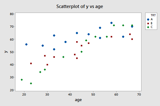
The blue circles represent the data for individuals receiving treatment A, the red squares represent the data for individuals receiving treatment B, and the green diamonds represent the data for individuals receiving treatment C.
In the previous example, the two estimated regression functions had the same slopes —that is, they were parallel. If you tried to draw three best-fitting lines through the data of this example, do you think the slopes of your lines would be the same? Probably not! In this case, we need to include what are called "interaction terms" in our formulated regression model.
A (second-order) multiple regression model with interaction terms is:
\(y_i=\beta_0+\beta_1x_{i1}+\beta_2x_{i2}+\beta_3x_{i3}+\beta_{12}x_{i1}x_{i2}+\beta_{13}x_{i1}x_{i3}+\epsilon_i\)
where:
- \(y_{i} =\) measure of the effectiveness of the treatment for individual i
- \(x_{i1} =\) age (in years) of individual i
- \(x_{i2} = 1\) if individual i received treatment A and 0, if not
- \(x_{i3} = 1\) if individual i received treatment B and 0, if not
and the independent error terms \(\epsilon_i\) follow a normal distribution with mean 0 and equal variance \(\sigma^{2}\). Perhaps not surprisingly, the terms \(x_{i} x_{i2}\) and \(x_{i1} x_{i3}\) are the interaction terms in the model.
Let's investigate our formulated model to discover in what way the predictors have an "interaction effect" on the response. We start by determining the formulated regression function for each of the three treatments. In short —after a little bit of algebra (see below) —we learn that the model defines three different regression functions —one for each of the three treatments:
| Treatment | Formulated regression function |
|---|---|
| If patient receives A, then \( \left(x_{i2} = 1, x_{i3} = 0 \right) \) and ... |
\(\mu_Y=(\beta_0+\beta_2)+(\beta_1+\beta_{12})x_{i1}\) |
| If patient receives B, then \( \left(x_{i2} = 0, x_{i3} = 1 \right) \) and ... |
\(\mu_Y=(\beta_0+\beta_3)+(\beta_1+\beta_{13})x_{i1}\) |
| If patient receives C, then \( \left(x_{i2} = 0, x_{i3} = 0 \right) \) and ... |
\(\mu_Y=\beta_0+\beta_{1}x_{i1}\) |
So, in what way does including the interaction terms, \(x_{i1} x_{i2}\) and \(x_{i1} x_{i3}\), in the model imply that the predictors have an "interaction effect" on the mean response? Note that the slopes of the three regression functions differ —the slope of the first line is \(\beta_1 + \beta_{12}\), the slope of the second line is \(\beta_1 + \beta_{13}\), and the slope of the third line is \(\beta_1\). What does this mean in a practical sense? It means that...
- the effect of the individual's age \(\left( x_1 \right)\) on the treatment's mean effectiveness \(\left(\mu_Y \right)\) depends on the treatment \(\left(x_2 \text{ and } x_3\right)\), and ...
- the effect of treatment \(\left(x_2 \text{ and } x_3\right)\) on the treatment's mean effectiveness \(\left(\mu_Y \right)\) depends on the individual's age \(\left( x_1 \right)\).
In general, then, what does it mean for two predictors "to interact"?
- Two predictors interact if the effect on the response variable of one predictor depends on the value of the other.
- A slope parameter can no longer be interpreted as the change in the mean response for each unit increase in the predictor, while the other predictors are held constant.
And, what are "interaction effects"?
A regression model contains interaction effects if the response function is not additive and cannot be written as a sum of functions of the predictor variables. That is, a regression model contains interaction effects if:
\(\mu_Y \ne f_1(x_1)+f_1(x_1)+ \cdots +f_{p-1}(x_{p-1})\)
For our example concerning treatment for depression, the mean response:
\(\mu_Y=\beta_0+\beta_1x_{1}+\beta_2x_{2}+\beta_3x_{3}+\beta_{12}x_{1}x_{2}+\beta_{13}x_{1}x_{3}\)
can not be separated into distinct functions of each of the individual predictors. That is, there is no way of "breaking apart" \(\beta_{12} x_1 x_2 \text{ and } \beta_{13} x_1 x_3\) into distinct pieces. Therefore, we say that \(x_1 \text{ and } x_2\) interact, and \(x_1 \text{ and } x_3\) interact.
In returning to our example, let's recall that the appropriate steps in any regression analysis are:
- Model building
- Model formulation
- Model estimation
- Model evaluation
- Model use
So far, within the model-building step, all we've done is formulate the regression model as:
\(y_i=\beta_0+\beta_1x_{i1}+\beta_2x_{i2}+\beta_3x_{i3}+\beta_{12}x_{i1}x_{i2}+\beta_{13}x_{i1}x_{i3}+\epsilon_i\)
We can use Minitab —or any other statistical software for that matter —to estimate the model. Doing so, Minitab reports:
Regression Equation
y = 6.21 + 1.0334 age + 41.30 x2+ 22.71 x3 - 0.703 agex2 - 0.510 agex3
Now, if we plug the possible values for \(x_2 \text{ and } x_3\) into the estimated regression function, we obtain the three "best fitting" lines —one for each treatment (A, B, and C) —through the data. Here's the algebra for determining the estimated regression function for patients receiving treatment A.
Doing similar algebra for patients receiving treatments B and C, we obtain:
| Treatment | Estimated regression function |
|---|---|
| If patient receives A, then \(\left(x_2 = 1, x_3 = 0 \right)\) and ... |
\(\hat{y}=47.5+0.33x_1\) |
| If patient receives B, then \(\left(x_2 = 0, x_3 = 1 \right)\) and ... |
\(\hat{y}=28.9+0.52x_1\) |
| If patient receives C, then \(\left(x_2 = 0, x_3 = 0 \right)\) and ... |
\(\hat{y}=6.21+1.03x_1\) |
And, plotting the three "best fitting" lines, we obtain:
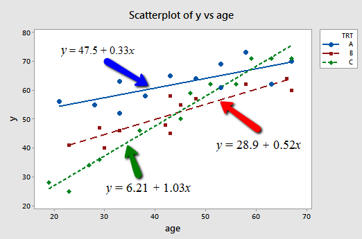
What do the estimated slopes tell us?
- For patients in this study receiving treatment A, the effectiveness of the treatment is predicted to increase by 0.33 units for every additional year in age.
- For patients in this study receiving treatment B, the effectiveness of the treatment is predicted to increase by 0.52 units for every additional year in age.
- For patients in this study receiving treatment C, the effectiveness of the treatment is predicted to increase by 1.03 units for every additional year in age.
In short, the effect of age on the predicted treatment effectiveness depends on the treatment given. That is, age appears to interact with treatment in its impact on treatment effectiveness. The interaction is exhibited graphically by the "nonparallelness" (is that a word?) of the lines.
Of course, our primary goal is not to draw conclusions about this particular sample of depressed individuals, but rather about the entire population of depressed individuals. That is, we want to use our estimated model to draw conclusions about the larger population of depressed individuals. Before we do so, however, we first should evaluate the model.
The residuals versus fits plot:
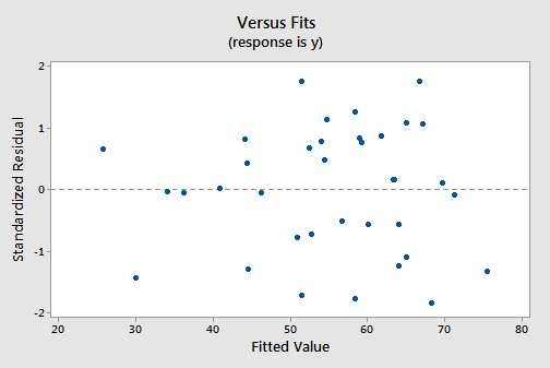
exhibits all of the "good" behavior, suggesting that the model fits well, there are no obvious outliers, and the error variances are indeed constant. And, the normal probability plot:
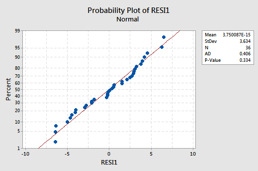
exhibits a linear trend and a large P-value, suggesting that the error terms are indeed normally distributed.
Having successfully built —formulated, estimated, and evaluated —a model, we now can use the model to answer our research questions. Let's consider two different questions that we might want to be answered.
First research question. For every age, is there a difference in the mean effectiveness for the three treatments? As is usually the case, our formulated regression model helps determine how to answer the research question. Our formulated regression model suggests that answering the question involves testing whether the population regression functions are identical.
That is, we need to test the null hypothesis \(H_0 \colon \beta_2 = \beta_3 =\beta_{12} = \beta_{13} = 0\) against the alternative \(H_A \colon\) at least one of these slope parameters is not 0.
We know how to do that! The relevant software output:
Analysis of Variance
| Source | DF | Seq SS | Seq MS | F-Value | P-Value |
|---|---|---|---|---|---|
| Regression | 5 | 4932.85 | 986.57 | 64.04 | 0.000 |
| age | 5 | 3424.43 | 3424.43 | 222.29 | 0.000 |
| x2 | 1 | 803.80 | 803.80 | 52.18 | 0.000 |
| x3 | 1 | 1.19 | 1.19 | 0.08 | 0.783 |
| agex2 | 1 | 375.00 | 375.00 | 24.34 | 0.000 |
| agex3 | 1 | 328.42 | 328.42 | 21.32 | 0.000 |
| Error | 30 | 462.15 | 15.40 | ||
| Lack-of-Fit | 27 | 285.15 | 10.56 | 0.18 | 0.996 |
| Pure Error | 3 | 177.00 | 59.00 | ||
| Total | 35 | 5395.0 |
tells us that the appropriate partial F-statistic for testing the above hypothesis is:
\(F=\frac{(803.8+1.19+375+328.42)/4}{15.4}=24.49\)
And, Minitab tells us:
F Distribution with 4 DF in Numerator and 30 DF in denominator
| x | \(p(X \leq x)\) |
|---|---|
| 24.49 | 1.00000 |
that the probability of observing an F-statistic —with 4 numerator and 30 denominator degrees of freedom —less than our observed test statistic 24.49 is > 0.999. Therefore, our P-value is < 0.001. We can reject our null hypothesis. There is sufficient evidence at the \(\alpha = 0.05\) level to conclude that there is a significant difference in the mean effectiveness for the three treatments.
Second research question. Does the effect of age on the treatment's effectiveness depend on the treatment? Our formulated regression model suggests that answering the question involves testing whether the two interaction parameters \(\beta_{12} \text{ and } \beta_{13}\) are significant. That is, we need to test the null hypothesis \(H_0 \colon \beta_{12} = \beta_{13} = 0\) against the alternative \(H_A \colon\) at least one of the interaction parameters is not 0.
The relevant software output:
Analysis of Variance
| Source | DF | Seq SS | Seq MS | F-Value | P-Value |
|---|---|---|---|---|---|
| Regression | 5 | 4932.85 | 986.57 | 64.04 | 0.000 |
| age | 5 | 3424.43 | 3424.43 | 222.29 | 0.000 |
| x2 | 1 | 803.80 | 803.80 | 52.18 | 0.000 |
| x3 | 1 | 1.19 | 1.19 | 0.08 | 0.783 |
| agex2 | 1 | 375.00 | 375.00 | 24.34 | 0.000 |
| agex3 | 1 | 328.42 | 328.42 | 21.32 | 0.000 |
| Error | 30 | 462.15 | 15.40 | ||
| Lack-of-Fit | 27 | 285.15 | 10.56 | 0.18 | 0.996 |
| Pure Error | 3 | 177.00 | 59.00 | ||
| Total | 35 | 5395.0 |
tells us that the appropriate partial F-statistic for testing the above hypothesis is:
\(F=\dfrac{(375+328.42)/2}{15.4}=22.84\)
And, Minitab tells us:
F Distribution with 2 DF in Numerator and 30 DF in denominator
| x | \(p(X \leq x)\) |
|---|---|
| 22.84 | 1.00000 |
that the probability of observing an F-statistic — with 2 numerator and 30 denominator degrees of freedom — less than our observed test statistic 22.84 is > 0.999. Therefore, our P-value is < 0.001. We can reject our null hypothesis. There is sufficient evidence at the \(\alpha = 0.05\) level to conclude that the effect of age on the treatment's effectiveness depends on the treatment.
Try It!
A model with an interaction term
-
For the depression study, plug the appropriate values for \(x_2 \text{ and } x_3\) into the formulated regression function and perform the necessary algebra to determine:
- The formulated regression function for patients receiving treatment B.
- The formulated regression function for patients receiving treatment C.
\(\mu_Y = \beta_0+\beta_1x1+\beta_2 x_2+\beta_3 x_3+\beta_{12}x_1 x_2+\beta_{13} x_1 x_3\)
\(\mu_Y = \beta_0+\beta_1 x_1+\beta_2(0)+\beta_3(1)+\beta_{12} x_1(0)+\beta_{13} x_1(1) = (\beta_0+\beta_3)+(\beta_1+\beta_{13})x_1\)
\(\mu_Y = \beta_0+\beta_1 x_1+\beta_2(0)+\beta_3(0)+\beta_{12} x_1(0)+\beta_{13} x_1(0) = \beta_0+\beta_1 x_1\)
-
Treatment B, \(x_2 = 0 , x_3 = 1\), so
-
Treatment C, \(x_2 = 0 , x_3 = 0\), so
-
For the depression study, plug the appropriate values for \(x_2 \text{ and } x_3\) into the estimated regression function and perform the necessary algebra to determine:
- The estimated regression function for patients receiving treatment B.
- The estimated regression function for patients receiving treatment C.
\(\hat{y} = 6.21 + 1.0334 x_1 + 41.30 x_2+22.71 x_3 - 0.703 x_1 x_2 - 0.510 x_1 x_3\)
\(\hat{y} = 6.21 + 1.0334 x_1 + 41.30(0) + 22.71(1) - 0.703 x_1(0) - 0.510 x_1(1) = (6.21 + 22.71)+(1.0334 - 0.510) x_1 = 28.92 + 0.523 x_1\)
\(\hat{y} = 6.21 + 1.0334 x_1 + 41.30(0) + 22.71(0) - 0.703 x_1(0) - 0.510 x_1(0) = 6.21 + 1.033 x_1\)
-
Treatment B, \(x_2 = 0 , x_3 = 1\), so
-
Treatment C, \(x_2 = 0 , x_3 = 0\), so
-
For the first research question that we addressed for the depression study, show that there is no difference in the mean effectiveness between treatments B and C, for all ages, provided that \(\beta_3 = 0 \text{ and } \beta_{13} = 0\). (HINT: Follow the argument presented in the chalk-talk comparing treatments A and C.)
\(\mu_Y|\text{Treatment B} - \mu_Y|\text{Treatment C} = (\beta_0 + \beta_3)+(\beta_1 + \beta_{13}) x_1 - (\beta_0 + \beta_1 x_1) = \beta_3 + \beta_{13} x_1 = 0\), if \(\beta_3 = \beta_{13} = 0\)
-
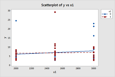
A study of atmospheric pollution on the slopes of the Blue Ridge Mountains (Tennessee) was conducted. The Lead Moss data contains the levels of lead found in 70 fern moss specimens (in micrograms of lead per gram of moss tissue) collected from the mountain slopes, as well as the elevation of the moss specimen (in feet) and the direction (1 if east, 0 if west) of the slope face.
- Write the equation of a second-order model relating mean lead level, E(y), to elevation \(\left(x_1 \right)\) and the slope face \(\left(x_2 \right)\) that includes an interaction between elevation and slope face in the model.
- Graph the relationship between mean lead level and elevation for the different slope faces that are hypothesized by the model in part a.
- In terms of the β's of the model in part a, give the change in lead level for every one-foot increase in elevation for moss specimens on the east slope.
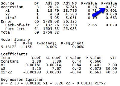
- Fit the model in part a to the data using an available statistical software package. Is the overall model statistically useful for predicting lead level? Test using \(α = 0.10\).
- Write the estimated equation of the model in part a relating mean lead level, E(y), to elevation \(\left(x_1 \right)\) and slope face \(\left(x_2 \right)\).
Since the p-value for testing whether the overall model is statistically useful for predicting lead level is 0.857, we conclude that this model is not statistically useful.
(e) The estimated equation is shown in the Minitab output above, but since the model is not statistically useful, this equation doesn’t do us much good.
-
\(\mu_Y = \beta_0 + \beta_1 x_1 + \beta_2 x_2 + \beta_{12} x_1 x_2\)
-
-
East slope, \(x_2=1\), \(\mu_Y = \beta_0 + \beta_1 x_1 + \beta_2(1) + \beta_{12} x_1(1) = (\beta_0 + \beta_2)+(\beta_1 + \beta_{12}) x_1\), so average lead level changes by \(\beta_1 + \beta_{12}\) micrograms of lead per gram of moss tissue for every one foot increase in elevation for moss specimens on the east slope.
-
8.7 - Leaving an Important Interaction Out of a Model
8.7 - Leaving an Important Interaction Out of a ModelImpact of Removing a Necessary Interaction Term out of the Model
Before we take a look at another example of a regression model containing interaction terms, let's take a little detour to explore the impact of leaving a necessary interaction term out of the model. To do so, let's consider some contrived data for which there is a response y and two predictors —one quantitative predictor x, and one qualitative predictor that takes on values 0 or 1. Looking at a plot of the data:
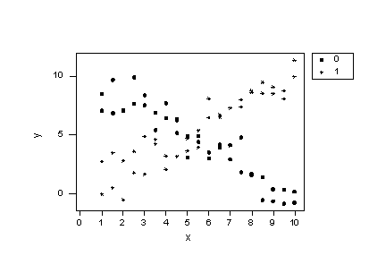
consider two questions:
-
Does the plot suggest that x is related to y? Sure! For the 0 group, as x increases, y decreases, while for the 1 group, as x increases, y also increases.
-
Does the plot suggest there is a treatment effect? Yes! If you look at any one particular x value, say 1 for example, the mean response y is about 8 for the 0 group and about 2 for the 1 group. In this sense, there is a treatment effect.
As we now know, the answer to the first question suggests that the effect of x on y depends on the group. That is, the group and x appear to interact. Therefore, our regression model should contain an interaction term between the two predictors. But, let's see what happens if we ignore our intuition and don't add the interaction term! That is, let's formulate our regression model as:
\(y_i=(\beta_0+\beta_1x_{i1}+\beta_2x_{i2})+\epsilon_i\)
where:
- \(y_i\) is the response
- \(x_{i1}\) is the quantitative predictor you want to "adjust for "
- \(x_{i2}\) is the qualitative group predictor, where 0 denotes the first group and 1 denotes the second group
and the independent error terms \(\epsilon_{i}\) follow a normal distribution with mean 0 and equal variance \(\sigma^{2}\).
Now, let's see what conclusions we draw when we fit our contrived data to our formulated model with no interaction term:
The Regression equation is y = 4.55 - 0.025 x + 1.10 group
| Predictor | Coef | SE Coef | T | P |
|---|---|---|---|---|
| Constant | 4.5492 | 0.8665 | 5.25 | 0.000 |
| x | -0.0276 | 0.1288 | -0.21 | 0.831 |
| group | 1.0959 | 0.7056 | 1.55 | 0.125 |
Analysis of Variance
| Source | DF | SS | MS | F | P |
|---|---|---|---|---|---|
| Regression | 2 | 23.255 | 11.628 | 1.23 | 0.298 |
| Residual Error | 73 | 690.453 | 9.458 | ||
| Total | 75 | 713.709 |
| Source | DF | Seq SS |
|---|---|---|
| x | 1 | 0.435 |
| group | 1 | 22.820 |
Consider our two research questions:
-
Is x related to y? Minitab reports that the P-value for testing \(H_0 \colon \beta_1 = 0 \text{ is } 0.831\). There is insufficient evidence at the 0.05 level to conclude that x is related to y. What?! This conclusion contradicts what we'd expect from the plot.
-
Is there a treatment effect? Minitab reports that the P-value for testing \(H_0 \colon \beta_2 = 0 \text{ is } 0.125\). There is insufficient evidence at the 0.05 level to conclude that there is a treatment effect. Again, this conclusion contradicts what we'd expect from the plot.
A side note. By conducting the above two tests independently, we increase our chance of making at least one Type I error. Since we are interested in answering both research questions, we could minimize our chance of making a Type I error by conducting the partial F-test for testing, \(H_0 \colon \beta_1 = \beta_2 = 0\), that is, that both parameters are simultaneously zero.
Now, let's try to understand why our conclusions don't agree with our intuition based on the plot. If we plug the values 0 and 1 into the group variable of the estimated regression equation we obtain two parallel lines —one for each group.
A plot of the resulting estimated regression functions:
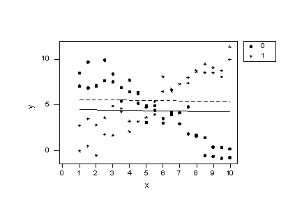
suggest that the lines don't fit the data very well. By leaving the interaction term out of the model, we have forced the "best fitting lines" to be parallel, when they clearly shouldn't be. The residuals versus fits plot:
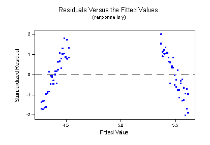
provides further evidence that our formulated model does not fit the data well. We now know that the resulting cost is conclusions that just don't make sense.
Let's analyze the data again, but this time with a more appropriately formulated model. Consider the regression model with the interaction term:
\(y_i=(\beta_0+\beta_1x_{i1}+\beta_2x_{i2}+\beta_{12}x_{i1}x_{i2})+\epsilon_i\)
where:
- \(y_i\) is the response
- \(x_{i1}\) is the quantitative predictor you want to "adjust for "
- \(x_{i2}\) is the qualitative group predictor, where 0 denotes the first group and 1 denotes the second group
- \(x_{i1}\)\(x_{i2}\) is the "missing" interaction term
and the independent error terms \(\epsilon_{i}\) follow a normal distribution with mean 0 and equal variance \(\sigma^{2}\).
Upon fitting the data to the model with an interaction term, Minitab reports:
Regression Equation
y = 10.1 - 1.04 x - 10.1 group + 2.03 groupxIf we now plug the values 0 and 1 into the group variable of the estimated regression equation we obtain two intersecting lines —one for each group:
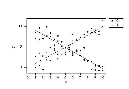
Wow —what a difference! Our formulated regression model now allows the slopes of the two lines to be different. As a result, the lines do a much better job of summarizing the trend in the data. The residuals versus fits plot is about as good as it gets!
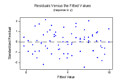
The plot provides further evidence that the model with the interaction term does a good job of describing the data.
Okay, so the model with the interaction term does a better job of describing the data than the model with no interaction term. Does it also provide answers to our research questions that make sense?
Let's first consider the question "does the effect of x on response y depend on the group?" That is, is there an interaction between x and the group? The Minitab output:
Regression Equation
y = 10.1 - 1.04 x - 10.1 group + 2.03 groupx
| Predictor | Coef | SE Coef | T | P |
|---|---|---|---|---|
| Constant | 10.1401 | 0.4320 | 23.47 | 0.000 |
| x | -1.04416 | 0.07031 | -14.85 | 0.000 |
| group | -10.0859 | 0.6110 | -16.51 | 0.000 |
| groupx | 2.03307 | 0.09944 | 20.45 | 0.000 |
| Model Summary | ||
|---|---|---|
| S = 1.187 | R-Sq = 85.8% | R-Sq(adj) = 85.2% |
Analysis of Variance
| Source | DF | SS | MS | F | P |
|---|---|---|---|---|---|
| Regression | 3 | 612.26 | 204.09 | 144.84 | 0.000 |
| Residual Error | 72 | 101.45 | 1.41 | ||
| Total | 75 | 713.71 |
tells us that the P-value for testing \(H_0 \colon \beta_{12} = 0 \text{ is } < 0.001\). There is strong evidence at the 0.05 level to reject the null hypothesis and conclude that there is indeed an interaction between x and the group. Aha —our formulated model and resulting analysis yielded a conclusion that makes sense!
Now, what about the research questions "is x related to y?" and "is there a treatment effect?" Because there is an interaction between x and the group, it doesn't make sense to talk about the effect of x on y without taking into account the group. And, it doesn't make sense to talk about differences in the two groups without taking into account x. That is, neither of these two research questions makes sense in the presence of the interaction. This is why you'll often hear statisticians say "never interpret the main effect in the presence of an interaction."
In short, the moral of the story of this little detour that we took is that if we leave an important interaction term out of our model, our analysis can lead us to make erroneous conclusions.
8.8 - Piecewise Linear Regression Models
8.8 - Piecewise Linear Regression ModelsExample 8-5: Piecewise linear regression model

We discuss what is called "piecewise linear regression models" here because they utilize interaction terms containing dummy variables.
Let's start with an example that demonstrates the need for using a piecewise approach to our linear regression model. Consider the following plot of the compressive strength (y) of n = 18 batches of concrete against the proportion of water (x) mixed in with the cement:
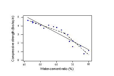
The estimated regression line —the solid line —appears to fit the data fairly well in some overall sense, but it is clear that we could do better. The residuals versus fits plot:
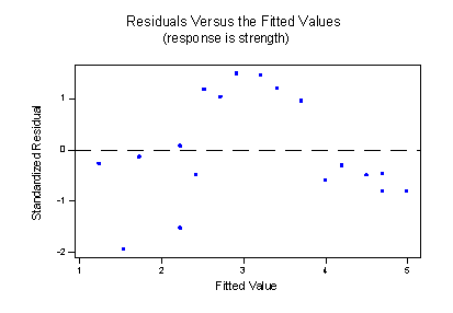
provides yet more evidence that our model needs work.
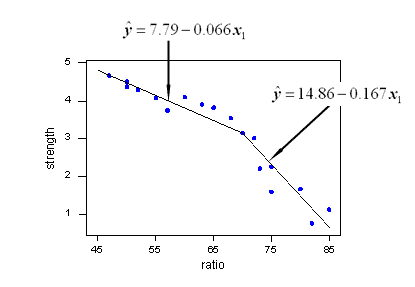
We could instead split our original scatter plot into two pieces —where the water-cement ratio is 70% —and fit two separate, but connected lines, one for each piece. As you can see, the estimated two-piece function, connected at 70% —the dashed line —appears to do a much better job of describing the trend in the data.
So, let's formulate a piecewise linear regression model for these data, in which there are two pieces connected at x = 70:
\(y_i=\beta_0+\beta_1x_{i1}+\beta_2(x_{i1}-70)x_{i2}+\epsilon_i\)
Alternatively, we could write our formulated piecewise model as:
\(y_i=\beta_0+\beta_1x_{i1}+\beta_2x_{i2}^{*}+\epsilon_i\)
where:
- \(y_i\) is the comprehensive strength, in pounds per square inch, of concrete batch i
- \(x_{i1}\) is the water-cement ratio, in %, of concrete batch i
- \(x_{i2}\) is a dummy variable \(\left( 0 , \text{ if } x_{i1} ≤ 70 \text{ and } 1 , \text{ if } x_{i1} > 70 \right)\) of concrete batch i
- \(x_{i2}*\) denotes the \(\left(x_{i1} - 70\right) x_{i2}\) the interaction term
and the independent error terms \(\epsilon_i\) follow a normal distribution with mean 0 and equal variance \(\sigma^{2}\).
With a little bit of algebra —
—we can see how the piecewise regression model as formulated above yields two separate linear functions connected at x = 70. Incidentally, the x-value at which the two pieces of the model connect is called the "knot value." For our example here, the knot value is 70.
Now, estimating our piecewise function in Minitab, we obtain:
The regression equation
strength = 7.79 - 0.0663 ratio - 0.101 x2*
| Predictor | Coef | SE Coef | T | P |
|---|---|---|---|---|
| Constant | 7.7920 | 0.6770 | 11.51 | 0.000 |
| ratio | -0.06633 | 0.01123 | -5.90 | 0.000 |
| x2* | -0.10119 | 0.02812 | -3.60 | 0.003 |
| Model Summary | ||
|---|---|---|
| S = 0.3286 | R-Sq = 93.8% | R-Sq(adj) = 93.0% |
Analysis of Variance
| Source | DF | SS | MS | F | P |
|---|---|---|---|---|---|
| Regression | 2 | 24.718 | 12.359 | 114.44 | 0.000 |
| Residual Error | 15 | 1.620 | 0.108 | ||
| Total | 17 | 26.338 |
With a little bit of algebra, we see how the estimated regression equation that Minitab reports:
Regression Equation
strength = 7.79 - 0.0663 ratio - 0.101 x2*yields two estimated regression lines, connected at x = 70, that fit the data quite well:
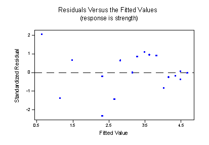
And, the residuals versus fits plot illustrates a significant improvement in the fit of the model:
Try It!
Piecewise linear regression
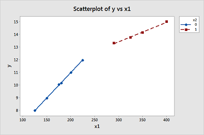
Shipment data. This exercise is intended to review the concept of piecewise linear regression. The basic idea behind piecewise linear regression is that if the data follow different linear trends over different regions of the data then we should model the regression function in "pieces." The pieces can be connected or not connected. Here, we'll fit a model in which the pieces are connected.
We'll use the Shipment dataset. An electronics company periodically imports shipments of a certain large part used as a component in several of its products. The size of the shipment varies depending on production schedules. For handling and distribution to assembly plants, shipments of size 250 thousand parts or less are sent to warehouse A; larger shipments are sent to warehouse B since this warehouse has specialized equipment that provides greater economies of scale for large shipments.
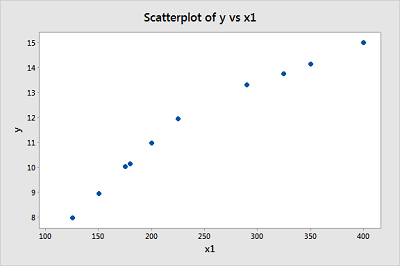
The data set contains information on the cost (y) of handling the shipment in the warehouse (in thousand dollars) and the size \(\left(x_1 \right)\) of the shipment (in thousand parts).
-
Create a scatter plot of the data with cost on the y-axis and size on the x-axis. (See Minitab Help: Creating a basic scatter plot). Based on the plot, does it seem reasonable that there are two different (but connected) regression functions — one when \(x_1 < 250\) and one when \(x_1 > 250\)?
-
Not surprisingly, we'll use a dummy variable and an interaction term to help define the piecewise linear regression model. Specifically, the model we'll fit is:
\(y_i = \beta_0 + \beta_1 x_{i1} + \beta_2 \left(x_{i1} - 250\right) x_{i2} + \epsilon_i\)
where \(x_{i1}\) is the size of the shipment and \(x_{i2} = 0\) if \(x_{i1} < 250\) and \(x_{i2} = 1\) if \(x_{i1} > 250\). We could also write this model as:
\(y_i = \beta0 + \beta_1 x_{i1} + \beta_2 {x^{*}}_{i2} + \epsilon_i\)
where \(x^*_{i2} = \left(x_{i1} - 250 \right) x_{i2}\). If we assume the data follow this model, what is the mean response function for shipments whose size is smaller than 250? And, what is the mean response function for shipments whose size is greater than 250? Do the two mean response functions have different slopes and connect when \(x_{i1} = 250\)?
\(\mu_Y = \beta_0 + \beta_1 x_1 + \beta_2 (x_1 - 250) x_2\)
\(\mu_Y|(x_1<250) = \beta_0 + \beta_1 x_1 + \beta_2 (x_1 - 250) (0) = \beta_0 + \beta_1 x_1\)
\(\mu_Y|(x_1>250) = \beta_0 + \beta_1 x_1 + \beta_2 (x_1 - 250) (1) = (\beta_0 - 250 \beta_2) + (\beta_1+\beta_2)x_1\)
When \(x_1=250, \beta_0 + \beta_1 x_1 = \beta_0 + 250\beta_1\)
When \(x_1=250, (\beta_0 - 250 \beta_2) + (\beta_1+\beta_2)(250) = \beta_0 + 250 \beta_1\)
-
You first need to set up the data set so that you can easily fit the model. In the data set, y denotes cost and \(x_1\) denotes the size. This is the easiest way to create the new variable, \(x*_{i2} = x_{1} ^{shift} x_2\), say:
- Use Minitab's calculator to create a new variable, \(x_1 ^{shift}\) , say, which equals \(x_1 - 250\).
- Use Minitab's Manip >> Code command (v16) or Data >> Recode >> To Numeric command (v17) to create \(x_2\). To do so, tell Minitab that you want to recode values in column x_{1} using the method "Recode range of values." Indicate that you want values from 0 to 250 to take on value 0 and values from 250 to 500 to take on value 1. Store the re-coded column in a specied column of the current worksheet named x2.
- Use Minitab's calculator to multiply \(x_1 ^{shift}\) by \(x_2\) to get \({x_1}^{shift} x_2\). Review the values obtained to convince yourself that they take on the values as defined. Then, fit the linear regression model with y as the response and \(x_1\) and \({x_1}^{shift} x_2\) as the predictors. What is the estimated regression function for shipments whose size < 250? for shipments whose size > 250?
\(\hat{y} = 3.214 + 0.038460 x_1 - 0.02477 x_1 \text{shift} x_2\)
\(\hat{y}|(x_1<250) = 3.214 + 0.038460 x_1 - 0.02477 (0) = 3.214 + 0.03846 x_1\)
\(\hat{y}|(x_1>250) = 3.214 + 0.038460 x_1 - 0.02477 (x_1-250) = (3.214 - 250(-0.02477)) + (0.038460-0.02477) x_1 = 9.4065 + 0.01369 x_1\)
-
Based on your estimated regression function, what is the predicted cost for a shipment with a size of 125? a size of 250? with a size of 400? Convince yourself that you get the same prediction for size = 250 regardless of which estimated regression function you use.
\(\hat{y}|(x_1=125) = 3.214 + 0.03846 (125) = 8.0215\)
\(\hat{y}|(x_1=250) = 3.214 + 0.03846 (250) = 12.8290\)
\(\hat{y}|(x_1=250) = 9.4065 + 0.01369 (250) = 12.8290\)
\(\hat{y}|(x_1=400) = 9.4065 + 0.01369 (400) = 14.8825\)
-
Using your predicted values for size = 125, 250, and 400, create another scatter plot of the data, but this time "annotate" the graph with the two connected lines. (Note that the F3 key should completely erase any previous work, such as annotation lines, in the Graph >> Plot command.) Do you think the piecewise linear regression model reasonably summarizes these data?
8.9 - Further Examples
8.9 - Further ExamplesExample 8-6: Additive Model
The Lesson8Ex1.txt dataset contains a response variable, Y, a quantitative predictor variable, X, and a categorical predictor variable, Cat, with three levels. We can code the information in Cat using two dummy indicator variables. A scatterplot of Y versus X with points marked by the level of Cat suggests three parallel regression lines with different intercepts but common slopes. We can confirm this with an F-test of the two X by dummy indicator variable interaction terms, which results in a high, non-significant p-value. We then refit without the interaction terms and confirm using individual t-tests that the intercept for level 2 differs from the intercept for level 1 and that the intercept for level 3 differs from the intercept for level 1.
Video Explanation
Example 8-7: Interaction Model
The Lesson8Ex2.txt dataset contains a response variable, Y, a quantitative predictor variable, X, and a categorical predictor variable, Cat, with three levels. We can code the information in Cat using two dummy indicator variables. A scatterplot of Y versus X with points marked by the level of Cat suggests three non-parallel regression lines with different intercepts and different slopes. We can confirm this with an F-test of the two X by dummy indicator variable interaction terms, which results in a low, significant p-value.
Video Explanation
Example 8-8: Muscle Mass Data
Suppose that we describe y = muscle mass as a function of \(x_1 = \text{ age and } x_2 = \text{ gender}\) for people in the 40 to 60 year-old age group. We could code the gender variable as \(x_2 = 1\) if the subject is female and \(x_2 = 0\) if the subject is male.
Consider the multiple regression equation
\(E\left(Y\right) = \beta_0 + \beta_1 x_1 + \beta_2 x_2\) .
The usual slope interpretation will work for \(\beta_2\), the coefficient that multiplies the gender indicator. Increasing gender by one unit simply moves us from male to female. Thus \(\beta_2\) = the difference between average muscle mass for females and males of the same age.
Example 8-9: Real Estate Air Conditioning
Consider the real estate dataset: Real estate data. Let us define
- \(Y =\) sale price of the home
- \(X_1 =\) square footage of home
- \(X_2 =\) whether the home has air conditioning or not.
To put the air conditioning variable into a model create a variable coded as either 1 or 0 to represent the presence or absence of air conditioning, respectively. With a 1, 0 coding for air conditioning and the model:
\(y_i = \beta_0 + \beta_1 x_{i,1} + \beta_2 x_{i,2} + \epsilon_i\)
the beta coefficient that multiplies the air conditioning variable will estimate the difference in average sale prices of homes that have air conditioning versus homes that do not, given that the homes have the same square foot area.
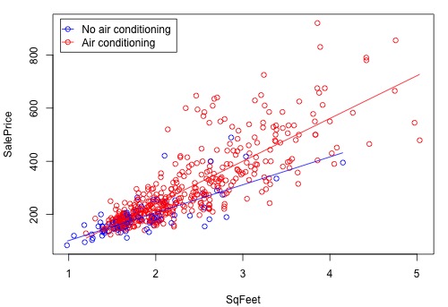
Suppose we think that the effect of air conditioning (yes or no) depends upon the size of the home. In other words, suppose that there is an interaction between the x-variables. To put an interaction into a model, we multiply the variables involved. The model here is
\(y_i = \beta_0 + \beta_1 x_{i,1} + \beta_2 x_{i,2} + \beta_3 x_{i,1}x_{i,2} + \epsilon_i\)
The data are from n = 521 homes. Statistical software output follows. Notice that there is a statistically significant result for the interaction term.
            Estimate Std. Error t value Pr(>|t|)
(Intercept)   -3.218     30.085  -0.107 0.914871
SqFeet       104.902     15.748   6.661 6.96e-11 ***
Air          -78.868     32.663  -2.415 0.016100 *
SqFeet.Air    55.888     16.580   3.371 0.000805 ***
The regression equation is:
Average SalePrice = −3.218 + 104.902 × SqrFeet − 78.868 × Air + 55.888 × SqrFeet × Air.
Suppose that a home has air conditioning. That means the variable Air = 1, so we’ll substitute Air = 1 in both places where Air occurs in the estimated model. This gives us
Average SalePrice = −3.218 + 104.902 × SqrFeet − 78.868(1) + 55.888 × SqrFeet × 1
= −82.086 + 160.790 × SqrFeet.
Suppose that a home does not have air conditioning. That means the variable Air = 0, so we’ll substitute Air = 0 in both places where Air occurs in the estimated model. This gives us
Average SalePrice = −3.218 + 104.902 × SqrFeet − 78.868(0) + 55.888 × SqrFeet × 0
= −3.218 + 104.902 × SqrFeet.
The figure below is a graph of the relationship between the sale price and square foot area for homes with air conditioning and homes without air conditioning. The equations of the two lines are the equations that we just derived above. The difference between the two lines increases as the square foot area increases. This means that the air conditioning versus no air conditioning difference in average sale price increases as the size of the home increases.
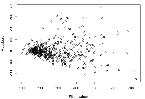
There is an increasing variance problem apparent in the above plot, which is even more obvious in the following residual plot:
We'll return to this example in Section 9.3 to see how to remedy this.
Example 8-10: Hospital Infection Risk Data
Consider the hospital infection risk data: Infection Risk data. For this example, the data are limited to observations with an average length of stay ≤ 14 days, which reduces the overall sample size to n = 111. The variables we will analyze are the following:
\(Y =\) infection risk in hospital
\(X_1 =\) average length of patient’s stay (in days)
\(X_2 =\) a measure of the frequency of giving X-rays
\(X_3 =\) indication in which of 4 U.S. regions the hospital is located (northeast, north-central, south, west).
The focus of the analysis will be on regional differences. The region is a categorical variable so we must use indicator variables to incorporate region information into the model. There are four regions. The full set of indicator variables for the four regions is as follows:
\(I_1 = 1\) if hospital is in region 1 (north-east) and 0 if not
\(I_2 = 1\) if hospital is in region 2 (north-central) and 0 if not
\(I_3 = 1\) if hospital is in region 3 (south) and 0 if not
\(I_4 = 1\) if hospital is in region 4 (west), 0 otherwise.
To avoid a linear dependency in the X matrix, we will leave out one of these indicators when we form the model. Using all but the first indicator to describe regional differences (so that "north-east" is the reference region), a possible multiple regression model for \(E\left(Y\right)\), the mean infection risk, is:
\( E \left(Y\right) = \beta_0 + \beta_1 X_1 + \beta_2 X_2 + \beta_3 I_2 + \beta_4 I_3 + \beta_5 I_4\)
To understand the meanings of the beta coefficients, consider each region separately:
- For hospitals in region 1 (north-east), \(I_2 = 0, I_3 = 0, \text{ and } I_4 = 0 \), so
\begin{align} E \left(Y\right) &= \beta_0 + \beta_1 X_1 + \beta_2 X_2 + \beta_3 \left(0\right) + \beta_4 \left(0\right) +\beta_5 \left(0\right)\\
&= \beta_0 + \beta_1 X_1 + \beta_2 X_2 \end{align}
- For hospitals in region 2 (north-central), \(I_2 = 1 , I_3 = 0, \text{ and } I_4 = 0\), so
\begin{align} E \left(Y\right) &= \beta_0 + \beta_1 X_1 + \beta_2 X_2 + \beta_3 (1) + \beta_4 \left(0\right) +\beta_5 \left(0\right)\\
&= \beta_0 + \beta_1 X_1 + \beta_2 X_2 + \beta_3 \end{align}
- For hospitals in region 3 (south), \(I_2 = 0, I_3 = 1, \text{ and } I_4 = 0 \), so
\begin{align} E \left(Y\right) &= \beta_0 + \beta_1 X_1 + \beta_2 X_2 + \beta_3 \left(0\right) + \beta_4 (1) +\beta_5 \left(0\right)\\
&= \beta_0 + \beta_1 X_1 + \beta_2 X_2 + \beta_4\end{align}
- For hospitals in region 4 (west), \(I_2 = 0, I_3 = 0, \text{ and } I_4 = 1 \), so
\begin{align} E \left(Y\right) &= \beta_0 + \beta_1 X_1 + \beta_2 X_2 + \beta_3 \left(0\right) + \beta_4 \left(0\right) +\beta_5 (1)\\
&= \beta_0 + \beta_1 X_1 + \beta_2 X_2 + \beta_5\end{align}
A comparison of the four equations just given provides these interpretations of the coefficients that multiply indicator variables:
- \(\beta_3 =\) difference in mean infection risk for region 2 (north-central) versus region 1 (north-east), assuming the same values for stay \(\left(X_1\right)\) and X-rays \(\left(X_2\right)\)
- \(\beta_4 =\) difference in mean infection risk for region 3 (south) versus region 1 (north-east), assuming the same values for stay \(\left(X_1\right)\) and X-rays \(\left(X_2\right)\)
- \(\beta_5 =\) difference in mean infection risk for region 4 (west) versus region 1 (north-east), assuming the same values for stay \(\left(X_1\right)\) and X-rays \(\left(X_2\right)\)
Estimate Std. Error t value Pr(>|t|)
(Intercept) -2.134259   0.877347  -2.433  0.01668 *
Stay         0.505394   0.081455   6.205 1.11e-08 ***
Xray         0.017587   0.005649   3.113  0.00238 **
i2           0.171284   0.281475   0.609  0.54416
i3           0.095461   0.288852   0.330  0.74169
i4           1.057835   0.378077   2.798  0.00612 **
---
Signif. codes:  0 ‘***’ 0.001 ‘**’ 0.01 ‘*’ 0.05 ‘.’ 0.1 ‘ ’ 1
Residual standard error: 1.036 on 105 degrees of freedom
Multiple R-squared:  0.4198,	Adjusted R-squared:  0.3922
F-statistic: 15.19 on 5 and 105 DF,  p-value: 3.243e-11
Some interpretations of results for individual variables are:
- We have statistical significance for the sample coefficient that multiplies \( I_4 \left(\text{p-value} = 0.006\right)\). This is the sample coefficient that estimates the coefficient \(\beta_5\), so we have evidence of a difference in the infection risks for hospitals in region 4 (west) and hospitals in region 1 (north-east), assuming the same values for stay (X1) and X-rays (X2). The positive coefficient indicates that the infection risk is higher in the west.
- The non-significance for the coefficients multiplying \( I_2 \text{ and } I_3\) indicates no observed difference between mean infection risks in region 2 (north-central) versus region 1 (north-east) nor between region 3 (south) versus region 1 (north-east), assuming the same values for stay (X1) and X-rays (X2).
Next, the finding of a difference between mean infection risks in the northeast and west seems to be strong, but for the sake of an example, we’ll now consider an overall test of regional differences. There is, in fact, an argument for doing so beyond “for the sake of example.” To assess regional differences, we considered three significance tests (for the three indicator variables). When we carry out multiple inferences, the overall error rate is increased so we may be concerned about a “fluke” result for one of the comparisons. If there are no regional differences, we would not have any indicator variables for regions in the model.
- The null hypothesis that makes this happen is \(H_0 \colon \beta_3 = \beta_4 = \beta_5 = 0\).
- The reduced model is simply \(E \left(Y\right) = \beta_0 + \beta_1 X_1 + \beta_2 X_2 \). This model has SSE = 123.56 with error df = 108.
- The full model is \(E \left(Y\right) = \beta_0 + \beta_1 X_1 + \beta_2 X_2 + \beta_3 I_2 + \beta_4 I_3 + \beta_5 I_4\), the model that we have already estimated. This model has SSE = 112.71 with error df = 105.
The test statistic for \(H_0 \colon \beta_3 = \beta_4 = \beta_5 = 0\) is the general linear F-statistic calculated as
\(F=\dfrac{\frac{\text{SSE(reduced) - SSE(full)}}{\text{error df for reduced - error df for full}}}{\text{MSE(full)}}=\dfrac{\frac{123.56-112.71}{108-105}}{\frac{112.71}{105}}=3.369.\)
The degrees of freedom for this F-statistic are 3 and 105. We find that the probability of getting an F statistic as extreme or more extreme than 3.369 under an \(F_{3,105}\) distribution is 0.021 (i.e., the p-value). We reject the null hypothesis and conclude that at least one of \(\beta_3\), \(\beta_4 , \text{ and } \beta_5 \) is not 0. Our previous look at the tests for individual coefficients showed us that it is \(\beta_5 \) (measuring the difference between west and northeast) that we conclude is different from 0.
Finally, the results seem to indicate that the west is the only regional difference we see that has a higher infection risk than the other three regions. (If the north-central and south regions don’t differ from the northeast, it is reasonable to think that they don’t differ from each other as well.) We can test this by considering a reduced model in which the only region indicator is \( I_4 = 1\) if west, and 0 otherwise. The model is
\(E \left(Y\right) = \beta_0 + \beta_1 X_1 + \beta_2 X_2 + \beta_5 I_4\).
The null hypothesis leading to this reduced model is \(H_0 \colon \beta_3 = \beta_4 = 0\). This model has SSE = 113.11 with error df = 107.
The full model is still
\(E \left(Y\right) = \beta_0 + \beta_1X_1 + \beta_2X_2 + \beta_3 I_1 + \beta_4 I_2 + \beta_5 I_3\),
which has SSE = 112.71 with error df = 105. Finally,
\(F=\dfrac{\frac{\text{SSE(reduced) - SSE(full)}}{\text{error df for reduced - error df for full}}}{\text{MSE(full)}}=\dfrac{\frac{113.11-112.71}{107-105}}{\frac{112.71}{105}}=0.186.\)
The degrees of freedom for this F-statistic are 2 and 105. We find that the probability of getting an F-statistic as extreme or more extreme than 0.186 under an \(F_{2,105}\) distribution is 0.831 (i.e., the p-value). Thus, we cannot reject the null hypothesis and conclude that the west difference from the other three regions seems to be reasonable.
8.10 - Summary
8.10 - SummaryIn this lesson, we briefly reviewed a multiple regression model that contained one binary predictor and one quantitative predictor and then went on to investigate such models more extensively. Although we primarily focused on models with a binary predictor, the methods and concepts extend readily to multiple regression models containing a general qualitative variable that, rather than defining just two groups, defines c groups.
We also learned how to formulate multiple regression models that contain "interaction effects" as a way to account for predictors that interact. We also investigated a special kind of model —called a "piecewise linear regression model" —that uses an interaction term as a way of creating a model that contains two or more different linear pieces.
Software Help 8
Software Help 8The next two pages cover the Minitab and commands for the procedures in this lesson.
Below is a zip file that contains all the data sets used in this lesson:
- birthsmokers.txt
- birthsmokers_02.txt
- depression.txt
- leadmoss.txt
- shipment
Minitab Help 8: Categorical Predictors
Minitab Help 8: Categorical PredictorsMinitab®
Birthweight and smoking (2-level categorical predictor, additive model)
- Create an indicator variable for Smoke by selecting Calc > Make Indicator Variables, move "Smoke" to the box labeled "Indicator variables for," and click "OK."
- Perform a linear regression analysis of Wgt on Gest + Smoke_yes. You can either put "Gest" and "Smoke_yes" in the box labeled "Continuous predictors" or, alternatively, put "Gest" in the box labeled "Continuous predictors" and "Smoke" in the box labeled "Categorical predictors." Either way, click "Storage" and select "Fits" before clicking "OK."
- Select Calc > Calculator, type "FITS0" in the box labeled "Store result in variable," type "if(Smoke="no",FITS)" in the box labeled "Expression," and click "OK." Repeat to create FITS1 as "if(Smoke="yes",FITS)."
- Create a basic scatterplot but select "With Groups" instead of "Simple." Plot "Wgt" vs "Gest" with "Smoke" as the "Categorical variable for grouping."
- To add parallel regression lines representing Smoke=0 and Smoke=1 to the scatterplot, select the scatterplot, select Editor > Add > Calculated Line, and select "FITS0" for the "Y column" and "Gest" for the "X column." Repeat to add the "FITS1" line.
- To display confidence intervals for the regression parameters, click "Results" in the Regression Dialog and select "Expanded tables" for "Display of results."
- Find a confidence interval and a prediction interval for the response to display confidence intervals for expected Wgt at Gest=38 (for Smoke=1 and Smoke=0).
- Select Data > Split Worksheet to create separate worksheets for Smoke=0 and Smoke=1.
- To repeat analysis using (1, -1) coding, click "Coding" in the Regression Dialog and select "(-1, 0, +1)" as the "Coding for categorical predictors."
Depression treatment (3-level categorical predictor, interaction model)
- Create a basic scatterplot but select "With Groups" instead of "Simple." Plot "y" (treatment effectiveness) vs "age" with "TRT" as the "Categorical variable for grouping."
- Perform a linear regression analysis of y on age (continuous) + TRT (categorical) but before clicking "OK," click "Model," select age and TRT together in the "Predictors" box, change "Interactions through order" to "2" and click "Add." You should see "age*TRT" appear in the box labeled "Terms in the model." Before clicking "OK," click "Coding," select "(1, 0)" for the "Coding for categorical predictors," and change the "Reference level" to "C."
- To add non-parallel regression lines representing each of the three treatments to the scatterplot do the following. Create a basic scatterplot but select "With Regression and Groups" instead of "Simple." Plot "y" (treatment effectiveness) vs "age" with "TRT" as the "Categorical variable for grouping."
- Create residual plots and select "Residuals versus fits" (with regular residuals).
- Conduct regression error normality tests and select Anderson-Darling.
- Click "Options" in the regression dialog to select Sequential (Type I) sums of squares to display an Anova table allowing calculation of F-statistic to see if at least one of x2, x3, age.x2, and age.x3 are useful (i.e., the regression functions differ).
- Use the same Anova table to calculate an F-statistic to see if at least one of age.x2 and age.x3 are useful (i.e., the regression functions have different slopes).
Real estate air conditioning (2-level categorical predictor, interaction model, transformations)
- Perform a linear regression analysis of SalePrice on SqFeet and Air (both continuous) but before clicking "OK," click "Model," select SqFeet and Air together in the "Predictors" box, change "Interactions through order" to "2" and click "Add." You should see "SqFeet*Air" appear in the box labeled "Terms in the model."
- To display a scatterplot of SalePrice vs SqFeet with points marked by Air and non-parallel regression lines representing Air=0 and Air=1 do the following. Create a basic scatterplot but select "With Regression and Groups" instead of "Simple." Plot "SalePrice" vs "SqFeet" with "Air" as the "Categorical variable for grouping."
- Create residual plots and select "Residuals versus fits" (with regular residuals).
- Select Calc > Calculator to create log(SalePrice) and log(SqFeet) variables and repeat preceding instructions to fit a multiple linear regression model of log(SalePrice) on log(SqFeet) + Air + log(SqFeet).Air.
- Repeat the preceding instructions to display a scatterplot of log(SalePrice) vs log(SqFeet) with points marked by Air and non-parallel regression lines representing Air=0 and Air=1.
- Create residual plots and select "Residuals versus fits" (with regular residuals).
Hospital infection risk (4-level categorical predictor, additive model)
- Use Data > Subset Worksheet to select only hospitals with Stay < 14.
- Perform a linear regression analysis of InfctRsk on Stay and Xray (continuous) and Region (categorical) but before clicking "OK," click "Coding," select "(1, 0)" for the "Coding for categorical predictors," and change the "Reference level" to "1."
- The resulting Anova table displays an F-statistic to see if at least one of i2, i3, and i4 is useful (conclusion: the regression functions differ by region).
- To calculate an F-statistic to see if at least one of i2 and i3 are useful you'll need to first create indicator variables for Region by selecting Calc > Make Indicator Variables. To find the reduced model results, Perform a linear regression analysis of InfctRsk on Stay, Xray, and Region_4 (all continuous).
R Help 8: Categorical Predictors
R Help 8: Categorical PredictorsR
Birthweight and smoking (2-level categorical predictor, additive model)
- Load the birthsmokers data.
- Create a scatterplot matrix of the data
- Fit a multiple linear regression model of Wgt on Gest + Smoke.
- Display scatterplot of Wgt vs Gest with points marked by Smoke and add parallel regression lines representing Smoke=0 and Smoke=1.
- Display regression results and calculate confidence intervals for the regression parameters.
- Display confidence intervals for expected Wgt at Gest=38 (for Smoke=1 and Smoke=0).
- Repeat analysis separately for Smoke=0 and Smoke=1.
- Repeat analysis using (1, -1) coding.
birthsmokers <- read.table("~/path-to-folder/birthsmokers.txt", header=T)
attach(birthsmokers)

pairs(cbind(Wgt, Gest, Smoke))

model <- lm(Wgt ~ Gest + Smoke)

plot(x=Gest, y=Wgt, ylim=c(2300, 3700),
     col=ifelse(Smoke=="yes", "red", "blue"),
     panel.last = c(lines(sort(Gest[Smoke=="no"]),
                          fitted(model)[Smoke=="no"][order(Gest[Smoke=="no"])],
                          col="blue"),
                    lines(sort(Gest[Smoke=="yes"]),
                          fitted(model)[Smoke=="yes"][order(Gest[Smoke=="yes"])],
                          col="red")))

summary(model)
#              Estimate Std. Error t value Pr(>|t|)
# (Intercept) -2389.573    349.206  -6.843 1.63e-07 ***
# Gest          143.100      9.128  15.677 1.07e-15 ***
# Smokeyes     -244.544     41.982  -5.825 2.58e-06 ***
# ---
# Residual standard error: 115.5 on 29 degrees of freedom
# Multiple R-squared:  0.8964,  Adjusted R-squared:  0.8892
# F-statistic: 125.4 on 2 and 29 DF,  p-value: 5.289e-15

confint(model)
#                  2.5 %     97.5 %
# (Intercept) -3103.7795 -1675.3663
# Gest          124.4312   161.7694
# Smokeyes     -330.4064  -158.6817

predict(model, interval="confidence",
        newdata=data.frame(Gest=c(38, 38), Smoke=c("yes", "no")))
#        fit      lwr      upr
# 1 2803.693 2740.599 2866.788
# 2 3048.237 2989.120 3107.355

model.0 <- lm(Wgt ~ Gest, subset=Smoke=="no")
summary(model.0)
#             Estimate Std. Error t value Pr(>|t|)
# (Intercept) -2546.14     457.29  -5.568 6.93e-05 ***
# Gest          147.21      11.97  12.294 6.85e-09 ***

predict(model.0, interval="confidence",
        newdata=data.frame(Gest=38))
#        fit      lwr     upr
# 1 3047.724 2990.298 3105.15

model.1 <- lm(Wgt ~ Gest, subset=Smoke=="yes")
summary(model.1)
#             Estimate Std. Error t value Pr(>|t|)
# (Intercept) -2474.56     553.97  -4.467 0.000532 ***
# Gest          139.03      14.11   9.851 1.12e-07 ***

predict(model.1, interval="confidence",
        newdata=data.frame(Gest=38))
#        fit      lwr      upr
# 1 2808.528 2731.726 2885.331

Smoke2 <- ifelse(Smoke=="yes", 1, -1)
model.3 <- lm(Wgt ~ Gest + Smoke2)
summary(model.3)
#              Estimate Std. Error t value Pr(>|t|)
# (Intercept) -2511.845    353.449  -7.107 8.07e-08 ***
# Gest          143.100      9.128  15.677 1.07e-15 ***
# Smoke2       -122.272     20.991  -5.825 2.58e-06 ***

# Alternatively
model.3 <- lm(Wgt ~ Gest + Smoke, contrasts=list(Smoke="contr.sum"))
summary(model.3)

detach(birthsmokers)
Depression treatments (3-level categorical predictor, interaction model)
- Load the depression data.
- Display scatterplot of y (treatment effectiveness) vs age with points marked by treatment.
- Create interaction variables and fit a multiple linear regression model of y on age + x2 + x3 + age.x2 + age.x3.
- Add non-parallel regression lines representing each of the three treatments to the scatterplot.
- Display a residuals vs fits plot and a normal probability plot of the residuals, and conduct an Anderson-Darling normality test using the
nortestpackage. - Conduct an F-test to see if at least one of x2, x3, age.x2, and age.x3 are useful (i.e., the regression functions differ).
- Conduct an F-test to see if at least one of age.x2 and age.x3 are useful (i.e., the regression functions have different slopes).
depression <- read.table("~/path-to-folder/depression.txt", header=T)
attach(depression)

plot(x=age, y=y, col=as.numeric(TRT))
legend("topleft", col=1:3, pch=1,
       inset=0.02, x.intersp = 1.5, y.intersp = 1.8,
       legend=c("Trt A", "Trt B", "Trt C"))

age.x2 <- age*x2
age.x3 <- age*x3

model.1 <- lm(y ~ age + x2 + x3 + age.x2 + age.x3)
summary(model.1)
#             Estimate Std. Error t value Pr(>|t|)
# (Intercept)  6.21138    3.34964   1.854 0.073545 .
# age          1.03339    0.07233  14.288 6.34e-15 ***
# x2          41.30421    5.08453   8.124 4.56e-09 ***
# x3          22.70682    5.09097   4.460 0.000106 ***
# age.x2      -0.70288    0.10896  -6.451 3.98e-07 ***
# age.x3      -0.50971    0.11039  -4.617 6.85e-05 ***

plot(x=age, y=y, ylim=c(20, 80), col=as.numeric(TRT),
     panel.last = c(lines(sort(age[TRT=="A"]),
                          fitted(model.1)[TRT=="A"][order(age[TRT=="A"])],
                          col=1),
                    lines(sort(age[TRT=="B"]),
                          fitted(model.1)[TRT=="B"][order(age[TRT=="B"])],
                          col=2),
                    lines(sort(age[TRT=="C"]),
                          fitted(model.1)[TRT=="C"][order(age[TRT=="C"])],
                          col=3)))
legend("topleft", col=1:3, pch=1, lty=1,
       inset=0.02, x.intersp = 1.5, y.intersp = 1.8,
       legend=c("Trt A", "Trt B", "Trt C"))

plot(x=fitted(model.1), y=rstudent(model.1),
     panel.last = abline(h=0, lty=2))

qqnorm(residuals(model.1), main="", datax=TRUE)
qqline(residuals(model.1), datax=TRUE)

library(nortest)
ad.test(residuals(model.1)) # A = 0.4057, p-value = 0.3345

anova(model.1)
#           Df Sum Sq Mean Sq  F value    Pr(>F)
# age        1 3424.4  3424.4 222.2946 2.059e-15 ***
# x2         1  803.8   803.8  52.1784 4.857e-08 ***
# x3         1    1.2     1.2   0.0772    0.7831
# age.x2     1  375.0   375.0  24.3430 2.808e-05 ***
# age.x3     1  328.4   328.4  21.3194 6.850e-05 ***
# Residuals 30  462.1    15.4

model.2 <- lm(y ~ age)
anova(model.2, model.1)
# Model 1: y ~ age
# Model 2: y ~ age + x2 + x3 + age.x2 + age.x3
#   Res.Df     RSS Df Sum of Sq     F    Pr(>F)
# 1     34 1970.57
# 2     30  462.15  4    1508.4 24.48 4.458e-09 ***

model.3 <- lm(y ~ age + x2 + x3)
anova(model.3, model.1)
# Model 1: y ~ age + x2 + x3
# Model 2: y ~ age + x2 + x3 + age.x2 + age.x3
#   Res.Df     RSS Df Sum of Sq      F   Pr(>F)
# 1     32 1165.57
# 2     30  462.15  2    703.43 22.831 9.41e-07 ***

detach(depression)
Real estate air conditioning (2-level categorical predictor, interaction model, transformations)
- Load the realestate data.
- Create an interaction variable and fit a multiple linear regression model of SalePrice on SqFeet + Air + SqFeet.Air.
- Display scatterplot of SalePrice vs SqFeet with points marked by Air and add non-parallel regression lines representing Air=0 and Air=1.
- Display residual plot with fitted (predicted) values on the horizontal axis.
- Create log(SalePrice), log(SqFeet), and log(SqFeet).Air variables and fit a multiple linear regression model of log(SalePrice) on log(SqFeet) + Air + log(SqFeet).Air.
- Display scatterplot of log(SalePrice) vs log(SqFeet) with points marked by Air and add non-parallel regression lines representing Air=0 and Air=1.
- Display residual plot with fitted (predicted) values on the horizontal axis.
realestate <- read.table("~/path-to-folder/realestate.txt", header=T)
attach(realestate)

SqFeet.Air <- SqFeet*Air
model.1 <- lm(SalePrice ~ SqFeet + Air + SqFeet.Air)
summary(model.1)
#             Estimate Std. Error t value Pr(>|t|)
# (Intercept)   -3.218     30.085  -0.107 0.914871
# SqFeet       104.902     15.748   6.661 6.96e-11 ***
# Air          -78.868     32.663  -2.415 0.016100 *
# SqFeet.Air    55.888     16.580   3.371 0.000805 ***

plot(x=SqFeet, y=SalePrice,
     col=ifelse(Air, "red", "blue"),
     panel.last = c(lines(sort(SqFeet[Air==0]),
                          fitted(model.1)[Air==0][order(SqFeet[Air==0])],
                          col="blue"),
                    lines(sort(SqFeet[Air==1]),
                          fitted(model.1)[Air==1][order(SqFeet[Air==1])],
                          col="red")))
legend("topleft", col=c("blue", "red"), pch=1, lty=1, inset=0.02,
       legend=c("No air conditioning", "Air conditioning"))

plot(x=fitted(model.1), y=residuals(model.1),
     xlab="Fitted values", ylab="Residuals",
     panel.last = abline(h=0, lty=2))

lnSalePrice <- log(SalePrice)
lnSqFeet <- log(SqFeet)
lnSqFeet.Air <- lnSqFeet*Air

model.2 <- lm(lnSalePrice ~ lnSqFeet + Air + lnSqFeet.Air)

plot(x=lnSqFeet, y=lnSalePrice,
     col=ifelse(Air, "red", "blue"),
     panel.last = c(lines(sort(lnSqFeet[Air==0]),
                          fitted(model.2)[Air==0][order(lnSqFeet[Air==0])],
                          col="blue"),
                    lines(sort(lnSqFeet[Air==1]),
                          fitted(model.2)[Air==1][order(lnSqFeet[Air==1])],
                          col="red")))
legend("topleft", col=c("blue", "red"), pch=1, lty=1, inset=0.02,
       legend=c("No air conditioning", "Air conditioning"))

plot(x=fitted(model.2), y=residuals(model.2),
     xlab="Fitted values", ylab="Residuals",
     panel.last = abline(h=0, lty=2))

detach(realestate)
Hospital infection risk (4-level categorical predictor, additive model)
- Load the infectionrisk data and select observations with Stay <= 14.
- Create indicator variables for regions.
- Fit a multiple linear regression model of InfctRsk on Stay + Xray + i2 + i3 + i4.
- Conduct an F-test to see if at least one of i2, i3, and i4 are useful (conclusion: the regression functions differ by region).
- Conduct an F-test to see if at least one of i2 and i3 are useful (conclusion: only the west region differs).
infectionrisk <- read.table("~/path-to-folder/infectionrisk.txt", header=T)
infectionrisk <- infectionrisk[infectionrisk$Stay<=14,]
attach(infectionrisk)

i1 <- ifelse(Region==1,1,0) # NE
i2 <- ifelse(Region==2,1,0) # NC
i3 <- ifelse(Region==3,1,0) # S
i4 <- ifelse(Region==4,1,0) # W

model.1 <- lm(InfctRsk ~ Stay + Xray + i2 + i3 + i4)
summary(model.1)
#              Estimate Std. Error t value Pr(>|t|)
# (Intercept) -2.134259   0.877347  -2.433  0.01668 *
# Stay         0.505394   0.081455   6.205 1.11e-08 ***
# Xray         0.017587   0.005649   3.113  0.00238 **
# i2           0.171284   0.281475   0.609  0.54416
# i3           0.095461   0.288852   0.330  0.74169
# i4           1.057835   0.378077   2.798  0.00612 **
# ---
# Residual standard error: 1.036 on 105 degrees of freedom
# Multiple R-squared:  0.4198,  Adjusted R-squared:  0.3922
# F-statistic: 15.19 on 5 and 105 DF,  p-value: 3.243e-11

model.2 <- lm(InfctRsk ~ Stay + Xray)
anova(model.2, model.1)
#   Res.Df    RSS Df Sum of Sq      F  Pr(>F)
# 1    108 123.56
# 2    105 112.71  3    10.849 3.3687 0.02135 *

model.3 <- lm(InfctRsk ~ Stay + Xray + i4)
anova(model.3, model.1)
#   Res.Df    RSS Df Sum of Sq      F Pr(>F)
# 1    107 113.11
# 2    105 112.71  2   0.39949 0.1861 0.8305

detach(infectionrisk)