In this section, we learn more about "leverages" and how they can help us identify extreme x values. We need to be able to identify extreme x values, because in certain situations they may highly influence the estimated regression function.

Definition and properties of leverages

You might recall from our brief study of the matrix formulation of regression that the regression model can be written succinctly as:

\[Y=X\beta+\epsilon\]

Therefore, the predicted responses can be represented in matrix notation as:

\[\hat{y}=Xb\]

And, if you recall that the estimated coefficients are represented in matrix notation as:

\[b = (X^{'}X)^{-1}X^{'}y\]

then you can see that the predicted responses can be alternatively written as:

\[\hat{y}=X(X^{'}X)^{-1}X^{'}y\]

That is, the predicted responses can be obtained by pre-multiplying the n × 1 column vector, y, containing the observed responses by the n × n matrix H:

\[H=X(X^{'}X)^{-1}X^{'}\]

That is:

\[\hat{y}=Hy\]

Do you see why statisticians call the n × n matrix H "the hat matrix?" That's right — because it's the matrix that puts the hat "ˆ" on the observed response vector y to get the predicted response vector \(\hat{y}\)! And, why do we care about the hat matrix? Because it contains the "leverages" that help us identify extreme x values!

If we actually perform the matrix multiplication on the right side of this equation:

\[\hat{y}=Hy\]

we can see that the predicted response for observation i can be written as a linear combination of the n observed responses y₁, y₂, ..., y_n:

\[\hat{y}_i=h_{i1}y_1+h_{i2}y_2+...+h_{ii}y_i+ ... + h_{in}y_n  \;\;\;\;\; \text{ for } i=1, ..., n\]

where the weights h_i1, h_i2, ..., h_ii, ..., h_in depend only on the predictor values. That is:

\(\hat{y}_1=h_{11}y_1+h_{12}y_2+\cdots+h_{1n}y_n\)
\(\hat{y}_2=h_{21}y_1+h_{22}y_2+\cdots+h_{2n}y_n\)
\(\vdots\)
\(\hat{y}_n=h_{n1}y_1+h_{n2}y_2+\cdots+h_{nn}y_n\)

Because the predicted response can be written as:

\[\hat{y}_i=h_{i1}y_1+h_{i2}y_2+...+h_{ii}y_i+ ... + h_{in}y_n  \;\;\;\;\; \text{ for } i=1, ..., n\]

the leverage, h_ii, quantifies the influence that the observed response y_i has on its predicted value \(\hat{y}_i\). That is, if h_ii is small, then the observed response y_i plays only a small role in the value of the predicted response \(\hat{y}_i\). On the other hand, if h_ii is large, then the observed response y_i plays a large role in the value of the predicted response \(\hat{y}_i\). It's for this reason that the h_ii are called the "leverages."

Here are some important properties of the leverages:

• The leverage h_ii is a measure of the distance between the x value for the i^th data point and the mean of the x values for all n data points.
• The leverage h_ii is a number between 0 and 1, inclusive.
• The sum of the h_ii equals k+1, the number of parameters (regression coefficients including the intercept).

The first bullet indicates that the leverage h_ii quantifies how far away the i^th x value is from the rest of the x values. If the i^th x value is far away, the leverage h_ii will be large; and otherwise not.

Let's use the above properties — in particular, the first one — to investigate a few examples.

Example #2 (again)

Let's take another look at the following data set (influence2.txt):

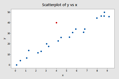
this time focusing only on whether any of the data points have high leverage on their predicted response. That is, are any of the leverages h_ii unusually high? What does your intuition tell you? Do any of the x values appear to be unusually far away from the bulk of the rest of the x values? Sure doesn't seem so, does it?

Let's see if our intuition agrees with the leverages. Rather than looking at a scatter plot of the data, let's look at a dotplot containing just the x values:

Three of the data points — the smallest x value, an x value near the mean, and the largest x value — are labeled with their corresponding leverages. As you can see, the two x values furthest away from the mean have the largest leverages (0.176 and 0.163), while the x value closest to the mean has a smaller leverage (0.048). In fact, if we look at a list of the leverages:

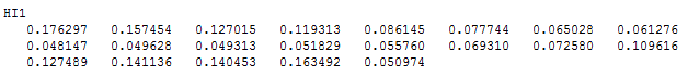
we see that as we move from the small x values to the x values near the mean, the leverages decrease. And, as we move from the x values near the mean to the large x values the leverages increase again (the last leverage in the list corresponds to the red point).

You might also note that the sum of all 21 of the leverages add up to 2, the number of beta parameters in the simple linear regression model — as we would expect based on the third property mentioned above.

Example #3 (again)

Let's take another look at the following data set (influence3.txt):

What does your intuition tell you here? Do any of the x values appear to be unusually far away from the bulk of the rest of the x values? Hey, quit laughing! Sure enough, it seems as if the red data point should have a high leverage value. Let's see!

A dotplot containing just the x values:

tells a different story this time. Again, of the three labeled data points, the two x values furthest away from the mean have the largest leverages (0.153 and 0.358), while the x value closest to the mean has a smaller leverage (0.048). Looking at a list of the leverages:

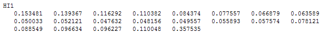
we again see that as we move from the small x values to the x values near the mean, the leverages decrease. And, as we move from the x values near the mean to the large x values the leverages increase again. But, note that this time, the leverage of the x value that is far removed from the remaining x values (0.358) is much, much larger than all of the remaining leverages. This leverage thing seems to work!

Oh, and don't forget to note again that the sum of all 21 of the leverages add up to 2, the number of beta parameters in the simple linear regression model. Again, we should expect this result based on the third property mentioned above.

Identifying data points whose x values are extreme

The great thing about leverages is that they can help us identify x values that are extreme and therefore potentially influential on our regression analysis. How? Well, all we need to do is determine when a leverage value should be considered large. A common rule is to flag any observation whose leverage value, h_ii, is more than 3 times larger than the mean leverage value:

\[\bar{h}=\frac{\sum_{i=1}^{n}h_{ii}}{n}=\frac{k+1}{n}\]

That is, if:

\[h_{ii} >3\left( \frac{k+1}{n}\right)\]

then flag the observations as "Unusual X" or "X denotes an observation whose X value gives it potentially large influence" or "X denotes an observation whose X value gives it large leverage").

As with many statistical "rules of thumb," not everyone agrees about this \(3 (k+1)/n\) cut-off and you may see \(2 (k+1)/n\) used as a cut-off instead. A refined rule of thumb that uses both cut-offs is to identify any observations with a leverage greater than \(3 (k+1)/n\) or, failing this, any observations with a leverage that is greater than \(2 (k+1)/n\) and very isolated.

Example #3 (again)

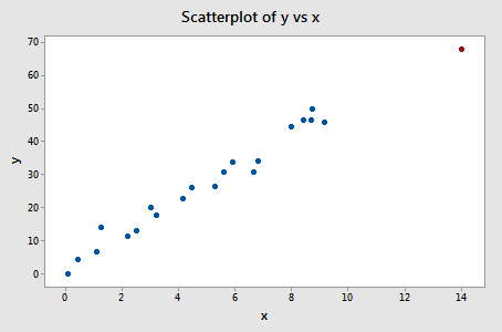
Let's try our leverage rule out an example or two, starting with this data set (influence3.txt):

Of course, our intution tells us that the red data point (x = 14, y = 68) is extreme with respect to the other x values. But, is the x value extreme enough to warrant flagging it? Let's see!

In this case, there are n = 21 data points and k+1 = 2 parameters (the intercept β₀ and slope β₁). Therefore:

\[3\left( \frac{k+1}{n}\right)=3\left( \frac{2}{21}\right)=0.286\]

Now, the leverage of the data point, 0.358, is greater than 0.286. Therefore, the data point should be flagged as having high leverage. And, that's exactly what happens in this statistical software output:

A word of caution! Remember, a data point has large influence only if it affects the estimated regression function. As we know from our investigation of this data set in the previous section, the red data point does not affect the estimated regression function all that much. Leverages only take into account the extremeness of the x values, but a high leverage observation may or may not actually be influential.

Example #4 (again)

Let's see how this the leverage rule works on this data set (influence4.txt):

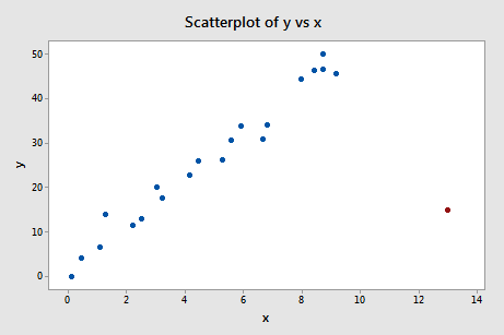
Of course, our intution tells us that the red data point (x = 13, y = 15) is extreme with respect to the other x values. Is the x value extreme enough to warrant flagging it?

Again, there are n = 21 data points and k+1 = 2 parameters (the intercept β₀ and slope β₁). Therefore:

\[3\left( \frac{k+1}{n}\right)=3\left( \frac{2}{21}\right)=0.286\]

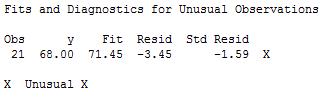
Now, the leverage of the data point, 0.311, is greater than 0.286. Therefore, the data point should be flagged as having high leverage, as it is:

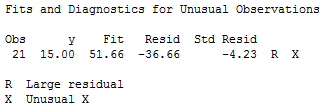
In this case, we know from our previous investigation that the red data point does indeed highly influence the estimated regression function. For reporting purposes, it would therefore be advisable to analyze the data twice — once with and once without the red data point — and to report the results of both analyses.

An important distinction!

There is such an important distinction between a data point that has high leverage and one that has high influence that it is worth saying it one more time:

• The leverage merely quantifies the potential for a data point to exert strong influence on the regression analysis.
• The leverage depends only on the predictor values.
• Whether the data point is influential or not also depends on the observed value of the reponse y_i.