In this section, we learn the following two measures for identifying influential data points:

• Difference in Fits (DFFITS)
• Cook's Distances

The basic idea behind each of these measures is the same, namely to delete the observations one at a time, each time refitting the regression model on the remaining n–1 observations. Then, we compare the results using all n observations to the results with the i^th observation deleted to see how much influence the observation has on the analysis. Analyzed as such, we are able to assess the potential impact each data point has on the regression analysis.

Difference in Fits (DFFITS)

The difference in fits for observation i, denoted DFFITS_i, is defined as:

\[DFFITS_i=\frac{\hat{y}_i-\hat{y}_{(i)}}{\sqrt{MSE_{(i)}h_{ii}}}\]

As you can see, the numerator measures the difference in the predicted responses obtained when the i^th data point is included and excluded from the analysis. The denominator is the estimated standard deviation of the difference in the predicted responses. Therefore, the difference in fits quantifies the number of standard deviations that the fitted value changes when the i^th data point is omitted.

An observation is deemed influential if the absolute value of its DFFITS value is greater than:

\[2\sqrt{\frac{k+2}{n-k-2}}\]

where, as always, n = the number of observations and k = the number of predictor terms (i.e., the number of regression parameters excluding the intercept). It is important to keep in mind that this is not a hard-and-fast rule, but rather a guideline only! It is not hard to find different authors using a slightly different guideline. Therefore, I often prefer a much more subjective guideline, such as a data point is deemed influential if the absolute value of its DFFITS value sticks out like a sore thumb from the other DFFITS values. Of course, this is a qualitative judgment, perhaps as it should be, since outliers by their very nature are subjective quantities.

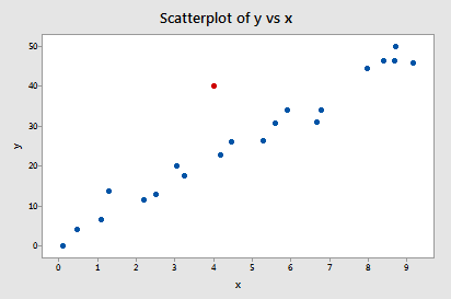
Example #2 (again). Let's check out the difference in fits measure for this data set (influence2.txt):

Regressing y on x and requesting the difference in fits, we obtain the following software output:

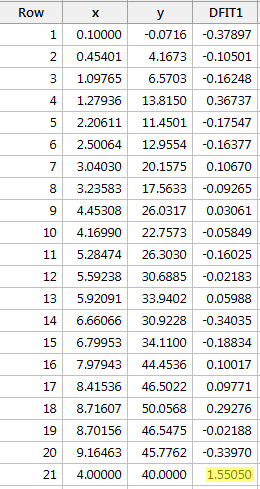
Using the objective guideline defined above, we deem a data point as being influential if the absolute value of its DFFITS value is greater than:

\[2\sqrt{\frac{k+2}{n-k-2}}=2\sqrt{\frac{1+2}{21-1-2}}=0.82.\]

Only one data point — the red one — has a DFFITS value whose absolute value (1.55050) is greater than 0.82. Therefore, based on this guideline, we would consider the red data point influential.

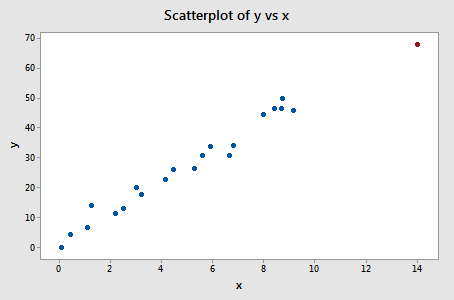
Example #3 (again). Let's check out the difference in fits measure for this data set (influence3.txt):

Regressing y on x and requesting the difference in fits, we obtain the following software output:

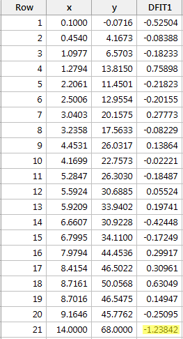
Using the objective guideline defined above, we deem a data point as being influential if the absolute value of its DFFITS value is greater than:

\[2\sqrt{\frac{k+2}{n-k-2}}=2\sqrt{\frac{1+1}{21-1-2}}=0.82.\]

Only one data point — the red one — has a DFFITS value whose absolute value (1.23841) is greater than 0.82. Therefore, based on this guideline, we would consider the red data point influential.

When we studied this data set in the beginning of this lesson, we decided that the red data point did not affect the regression analysis all that much. Yet, here, the difference in fits measure suggests that it is indeed influential. What is going on here? It all comes down to recognizing that all of the measures in this lesson are just tools that flag potentially influential data points for the data analyst. In the end, the analyst should analyze the data set twice — once with and once without the flagged data points. If the data points significantly alter the outcome of the regression analysis, then the researcher should report the results of both analyses.

Incidentally, in this example here, if we use the more subjective guideline of whether the absolute value of the DFFITS value sticks out like a sore thumb, we are likely not to deem the red data point as being influential. After all, the next largest DFFITS value (in absolute value) is 0.75898. This DFFITS value is not all that different from the DFFITS value of our "influential" data point.

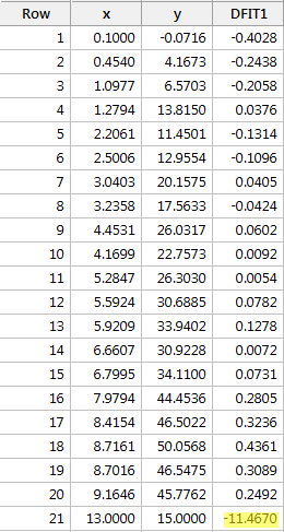
Example #4 (again). Let's check out the difference in fits measure for this data set (influence4.txt):

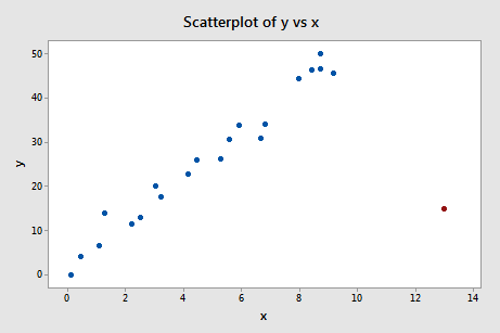
Regressing y on x and requesting the difference in fits, we obtain the following software output:

Using the objective guideline defined above, we again deem a data point as being influential if the absolute value of its DFFITS value is greater than:

\[2\sqrt{\frac{k+2}{n-k-2}}=2\sqrt{\frac{1+1}{21-1-2}}=0.82.\]

What do you think? Do any of the DFFITS values stick out like a sore thumb? Errr — the DFFITS value of the red data point (–11.4670 ) is certainly of a different magnitude than all of the others. In this case, there should be little doubt that the red data point is influential!

Cook's Distance

Just jumping right in here, Cook's distance measure, denoted D_i, is defined as:

\[D_i=\frac{(y_i-\hat{y}_i)^2}{(k+1) \times MSE}\left[ \frac{h_{ii}}{(1-h_{ii})^2}\right].\]

It looks a little messy, but the main thing to recognize is that Cook's D_i depends on both the residual, e_i (in the first term), and the leverage, h_ii (in the second term). That is, both the x value and the y value of the data point play a role in the calculation of Cook's distance.

In short:

• D_i directly summarizes how much all of the fitted values change when the i^th observation is deleted.
• A data point having a large D_i indicates that the data point strongly influences the fitted values.

Let's investigate what exactly that first statement means in the context of some of our examples.

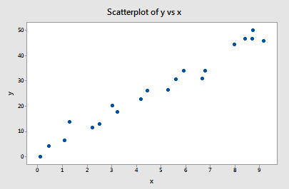
Example #1 (again). You may recall that the plot of these data (influence1.txt) suggests that there are no outliers nor influential data points for this example:

If we regress y on x using all n = 20 data points, we determine that the estimated intercept coefficient b₀ = 1.732 and the estimated slope coefficient b₁ = 5.117. If we remove the first data point from the data set, and regress y on x using the remaining n = 19 data points, we determine that the estimated intercept coefficient b₀ = 1.732 and the estimated slope coefficient b₁ = 5.1169. As we would hope and expect, the estimates don't change all that much when removing the one data point. Continuing this process of removing each data point one at a time, and plotting the resulting estimated slopes (b₁) versus estimated intercepts (b₀), we obtain:

The solid black point represents the estimated coefficients based on all n = 20 data points. The open circles represent each of the estimated coefficients obtained when deleting each data point one at a time. As you can see, the estimated coefficients are all bunched together regardless of which, if any, data point is removed. This suggests that no data point unduly influences the estimated regression function or, in turn, the fitted values. In this case, we would expect all of the Cook's distance measures, D_i, to be small.

Example #4 (again). You may recall that the plot of these data (influence4.txt) suggests that one data point is influential and an outlier for this example:

If we regress y on x using all n = 21 data points, we determine that the estimated intercept coefficient b₀ = 8.51 and the estimated slope coefficient b₁ = 3.32. If we remove the red data point from the data set, and regress y on x using the remaining n = 20 data points, we determine that the estimated intercept coefficient b₀ = 1.732 and the estimated slope coefficient b₁ = 5.1169. Wow—the estimates change substantially upon removing the one data point. Continuing this process of removing each data point one at a time, and plotting the resulting estimated slopes (b₁) versus estimated intercepts (b₀), we obtain:

Again, the solid black point represents the estimated coefficients based on all n = 21 data points. The open circles represent each of the estimated coefficients obtained when deleting each data point one at a time. As you can see, with the exception of the red data point (x = 13, y = 15), the estimated coefficients are all bunched together regardless of which, if any, data point is removed. This suggests that the red data point is the only data point that unduly influences the estimated regression function and, in turn, the fitted values. In this case, we would expect the Cook's distance measure, D_i, for the red data point to be large and the Cook's distance measures, D_i, for the remaining data points to be small.

Using Cook's distance measures. The beauty of the above examples is the ability to see what is going on with simple plots. Unfortunately, we can't rely on simple plots in the case of multiple regression. Instead, we must rely on guidelines for deciding when a Cook's distance measure is large enough to warrant treating a data point as influential.

Here are the guidelines commonly used:

• If D_i is greater than 0.5, then the i^th data point is worthy of further investigation as it may be influential.
• If D_i is greater than 1, then the i^th data point is quite likely to be influential.
• Or, if D_i sticks out like a sore thumb from the other D_i values, it is almost certainly influential.

Example #2 (again). Let's check out the Cook's distance measure for this data set (influence2.txt):

Regressing y on x and requesting the Cook's distance measures, we obtain the following software output:

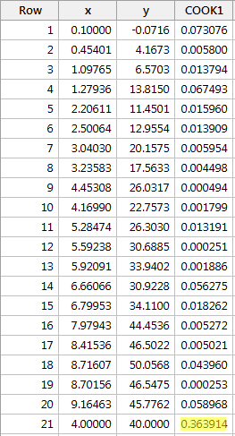
The Cook's distance measure for the red data point (0.363914) stands out a bit compared to the other Cook's distance measures. Still, the Cook's distance measure for the red data point is less than 0.5. Therefore, based on the Cook's distance measure, we would not classify the red data point as being influential.

Example #3 (again). Let's check out the Cook's distance measure for this data set (influence3.txt):

Regressing y on x and requesting the Cook's distance measures, we obtain the following software output:

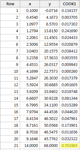
The Cook's distance measure for the red data point (0.701965) stands out a bit compared to the other Cook's distance measures. Still, the Cook's distance measure for the red data point is gretaer than 0.5 but less than 1. Therefore, based on the Cook's distance measure, we would perhaps investigate further but not necessarily classify the red data point as being influential.

Example #4 (again). Let's check out the Cook's distance measure for this data set (influence4.txt):

Regressing y on x and requesting the Cook's distance measures, we obtain the following software output:

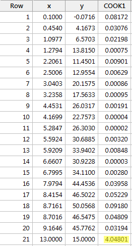
In this case, the Cook's distance measure for the red data point (4.04801) stands out substantially compared to the other Cook's distance measures. Furthermore, the Cook's distance measure for the red data point is greater than 1. Therefore, based on the Cook's distance measure—and not surprisingly—we would classify the red data point as being influential.

An alternative method for interpreting Cook's distance that is sometimes used is to relate the measure to the F(k+1, n–k–1) distribution and to find the corresponding percentile value. If this percentile is less than about 10 or 20 percent, then the case has little apparent influence on the fitted values. On the other hand, if it is near 50 percent or even higher, then the case has a major influence. (Anything "in between" is more ambiguous.)