So far, we have learned various measures for identifying extreme x values (high leverage observations) and unusual y values (outliers). When trying to identify outliers, one problem that can arise is when there is a potential outlier that influences the regression model to such an extent that the estimated regression function is "pulled" towards the potential outlier, so that it isn't flagged as an outlier using the standardized residual criterion. To address this issue, studentized residuals offer an alternative criterion for identifying outliers. The basic idea is to delete the observations one at a time, each time refitting the regression model on the remaining n–1 observations. Then, we compare the observed response values to their fitted values based on the models with the i^th observation deleted. This produces deleted residuals. Standardizing the deleted residuals produces studentized residuals.

Deleted Residuals

If we let:

• y_i denote the observed response for the i^th observation, and
• \(\hat{y}_{(i)}\) denote the predicted response for the i^th observation based on the estimated model with the i^th observation deleted

then the i^th (unstandardized) deleted residual is defined as:

\[d_i=y_i-\hat{y}_{(i)}\]

Why this measure? Well, data point i being influential implies that the data point "pulls" the estimated regression line towards itself. In that case, the observed response would be close to the predicted response. But, if you removed the influential data point from the data set, then the estimated regression line would "bounce back" away from the observed response, thereby resulting in a large deleted residual. That is, a data point having a large deleted residual suggests that the data point is influential.

An example. Consider the following plot of n = 4 data points (3 blue and 1 red):

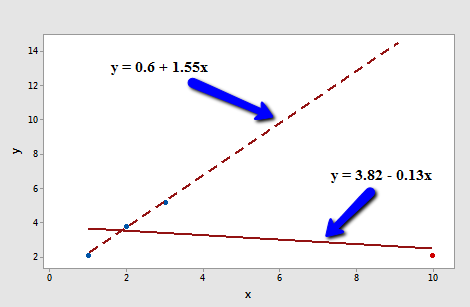
The solid line represents the estimated regression line for all four data points, while the dashed line represents the estimated regression line for the data set containing just the three data points — with the red data point omitted. Observe that, as expected, the red data point "pulls" the estimated regression line towards it. When the red data point is omitted, the estimated regression line "bounces back" away from the point.

Let's determine the deleted residual for the fourth data point — the red one. The value of the observed response is y₄ = 2.1. The estimated regression equation for the data set containing just the first three points is:

\[\hat{y}_{(4)}=0.6+1.55x\]

making the predicted response when x = 10:

\[\hat{y}_{(4)}=0.6+1.55(10)=16.1\]

Therefore, the deleted residual for the red data point is:

\[d_4=2.1-16.1=-14\]

Is this a large deleted residual? Well, we can tell from the plot in this simple linear regression case that the red data point is clearly influential, and so this deleted residual must be considered large. But, in general, how large is large? Unfortunately, there's not a straightforward answer to that question. Deleted residuals depend on the units of measurement just as the ordinary residuals do. We can solve this problem though by dividing each deleted residual by an estimate of its standard deviation. That's where "studentized residuals" come into play.

Studentized Residuals

A studentized residual (sometimes referred to as an "externally studentized residual" or a "deleted t residual") is:

\[t_i=\frac{d_i}{s(d_i)}=\frac{e_i}{\sqrt{MSE_{(i)}(1-h_{ii})}}\]

That is, a studentized residual is just a deleted residual divided by its estimated standard deviation (first formula). This turns out to be equivalent to the ordinary residual divided by a factor that includes the mean square error based on the estimated model with the i^th observation deleted, MSE_(i), and the leverage, h_ii (second formula). Note that the only difference between the standardized residuals considered in the previous section and the studentized residuals considered here is that standardized residuals use the mean square error for the model based on all observations, MSE, while studentized residuals use the mean square error based on the estimated model with the i^th observation deleted, MSE_(i),.

Another formula for studentized residuals allows them to be calculated using only the results for the model fit to all the observations:

\[t_i=r_i \left( \frac{n-k-2}{n-k-1-r_{i}^{2}}\right) ^{1/2},\]

where \(r_i\) is the i^th standardized residual, n = the number of observations, and k = the number of predictors.

In general, studentized residuals are going to be more effective for detecting outlying Y observations than standardized residuals. If an observation has a studentized residual that is larger than 3 (in absolute value) we can call it an outlier. [Recall from the previous section that some use the term "outlier" for an observation with a standardized residual that is larger than 3 in absolute value. To avoid any confusion, you should always clarify whether you're talking about standardized or studentized residuals when designating an observation to be an outlier.]

An example. Let's return to our example with n = 4 data points (3 blue and 1 red):

Regressing y on x and requesting the studentized residuals, we obtain the following software output:

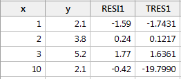
As you can see, the studentized residual ("TRES1") for the red data point is t₄ = -19.7990. Now we just have to decide if this is large enough to deem the data point influential. To do that we rely on the fact that, in general, studentized residuals follow a t distribution with (n–k–2) degrees of freedom. That is, all we need to do is compare the studentized residuals to the t distribution with (n–k–2) degrees of freedom. If a data point's studentized residual is extreme—that is, it sticks out like a sore thumb—then the data point is deemed influential.

Here, n = 4 and k = 1. Therefore, the t distribution has 4 – 1 – 2 = 1 degree of freedom. Looking at a plot of the t distribution with 1 degree of freedom:

we see that almost all of the t values for this distribution fall between -4 and 4. Three of the studentized residuals — –1.7431, 0.1217, and, 1.6361 — are all reasonable values for this distribution. But, the studentized residual for the fourth (red) data point (–19.799) sticks out like a very sore thumb. It is "off the chart" so to speak. Based on studentized residuals, the red data point is deemed influential.

Another example. Let's return to the Example #2 data set (influence2.txt):

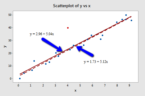
Regressing y on x and requesting the studentized residuals, we obtain the following software output:

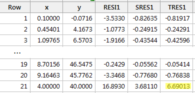
For the sake of saving space, I intentionally only show the output for the first three and last three observations. Again, the studentized residuals appear in the column labeled "TRES1." The studentized residual for the red data point is t₂₁ = 6.69013.

Because n–k–2 = 21–1–2 = 18, in order to determine if the red data point is influential, we compare the studentized residual to a t distribution with 18 degrees of freedom:

The studentized residual for the red data point (6.69013) sticks out like a sore thumb. Again, it is "off the chart." Based on studentized residuals, the red data point in this example is deemed influential. Incidentally, recall that earlier in this lesson, we deemed the red data point not influential for this example because it did not affect the estimated regression equation all that much. On the other hand, the red data point did substantially inflate the mean square error. Perhaps it is in this sense that one would want to treat the red data point as influential.