9.6 - Further Examples with Influential Points
Example 1: Male Foot Length and Height Data
First let us consider a dataset where y = foot length (cm) and x = height (in) for n = 33 male students in a statistics class (height_foot.txt). A scatterplot of the male foot length and height data shows one point labeled as an outlier:
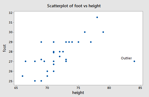
There is a clear outlier with values (xi , yi) = (84, 27). If that data point is deleted from the dataset, the estimated equation, using the other 32 data points, is \(\hat{y}_i = 0.253 + 0.384x_i\). For the deleted observation, xi = 84, so
\[\hat{y}_{i(i)}= 0.253 + 0.384(84) = 32.5093\]
The (unstandardized) deleted residual is
\[d_i=y_i-\hat{y}_{i(i)}= 27 − 32.5093 = −5.5093\]
The usual sample residual will be smaller in absolute size because the outlier will pull the line toward itself. With all data points used, \(\hat{y}_i = 10.936+0.2344x_i\). At xi = 84, \(\hat{y}_i = 30.5447\) and ei = 27 − 30.5447 = −3.5447.
The difference between the two predicted values computed for the outlier is:
unstandardized \(DFFITS = \hat{y}_i -\hat{y}_{i(i)}= 30.5447 − 32.5093 = −1.9646\).
Since √MSE(i)=1.028 and √hii=√0.356593=0.597, standardized DFFITS = –1.9646/(1.028*0.597) = –3.200.
A dotplot of Cook’s Di values for the male foot length and height data is below:
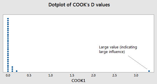
The one large value of Cook’s Di is for the point that is the outlier in the original data set. The interpretation is that the inclusion (or deletion) of this point will have a large influence on the overall results (which we saw from the calculations earlier).
From the analysis we did on the residuals, one may justify deleting the data point (xi , yi) = (84, 27) from the dataset. If you choose to take such a measure in practice, you need to always justify with some sort of residual analysis why you are deleting a data point.
Example 2: Hospital Infection Risk Data
 Below is a scatterplot for the hospital infection risk data (infectionrisk.txt).
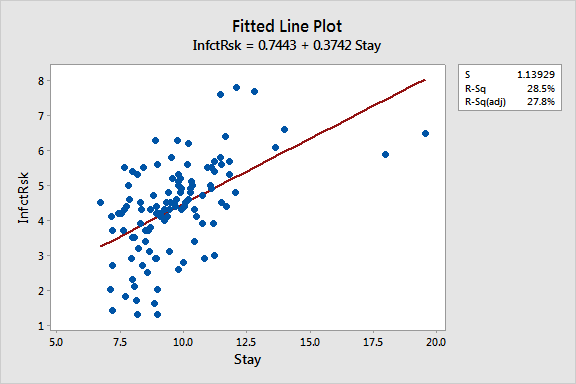
For this dataset, y = infection risk and x = average length of patient stay for n = 113 hospitals in the United States. A regression line is superimposed. Notice that there are two hospitals with extremely large values for length of stay and that the infection risks for those two hospitals are not correspondingly large. This causes the sample regression line to tilt toward the outliers and apparently not have the correct slope for the bulk of the data.
Below is list of “Unusual Observations” for this regression.
Fits and Diagnostics for Unusual Observations

Obs  InfctRsk    Fit  SE Fit      95% CI       Resid  Std Resid  Del Resid
  2     1.600  4.045   0.117  (3.813, 4.277)  -2.445      -2.16      -2.19
 40     1.300  3.798   0.136  (3.528, 4.068)  -2.498      -2.21      -2.25
 47     6.500  8.064   0.568  (6.938, 9.190)  -1.564      -1.58      -1.59
 53     7.600  5.014   0.146  (4.725, 5.304)   2.586       2.29       2.33
 54     7.800  5.261   0.173  (4.917, 5.605)   2.539       2.25       2.30
 93     1.300  4.082   0.115  (3.855, 4.310)  -2.782      -2.45      -2.51
104     6.600  5.965   0.265  (5.440, 6.490)   0.635       0.57       0.57
112     5.900  7.458   0.479  (6.508, 8.407)  -1.558      -1.51      -1.52

Obs        HI  Cook’s D      DFITS
  2  0.010526      0.02  -0.226306  R
 40  0.014263      0.04  -0.270442  R
 47  0.248925      0.42  -0.918229     X
 53  0.016434      0.04   0.301698  R
 54  0.023181      0.06   0.353981  R
 93  0.010146      0.03  -0.254391  R
104  0.054069      0.01   0.136676     X
112  0.176861      0.24  -0.702641     X

R  Large residual
X  Unusual X
Notice that three observations in this display are marked with an "X." Of these, observations 47 and 112 are the hospitals with the longest average length of stay. Notice also that these two points do not have particularly large standardized residuals ("Std Resid"). This is because the line was "pulled" toward the observed y-values and so the standardized residuals are not overly large. Also, these two points do not have particularly large studentized residuals ("Del Resid"). This is because studentized residuals only adjust for one observation being omitted from the model at a time. In this case, if Obs 47 is omitted, Obs 112 remains to "pull" the regression line towards its observed y-value. Similarly, if Obs 112 is omitted, Obs 47 remains to "pull" the regression line towards its observed y-value. Thus, the studentized residuals are unable to flag that these two observations are probably outliers.
There are five observations marked with an "R" for "large standardized residual." This is about the right number for a sample of n = 113 (5% of 113 comes to 5.65 observations) and none of these standardized residuals is overly large (say, greater than 3 in absolute value). Thus, the two data points to the far right are probably the only ones we need to worry about.
The question here would be whether we should delete the two hospitals to the far right and continue to use a linear model or whether we should retain the hospitals and use a curved model. The justification for deletion might be that we could limit our analysis to hospitals for which length of stay is less than 14 days, so we have a well defined criterion for the dataset that we use.

