One simple nonlinear model is the exponential regression model

\[\begin{equation*}
y_{i}=\beta_{0}+\beta_{1}\exp(\beta_{2}x_{i,1}+\ldots+\beta_{k+1}x_{i,k})+\epsilon_{i},
\end{equation*}\]

where the \(\epsilon_{i}\) are iid normal with mean 0 and constant variance \(\sigma^{2}\). Notice that if \(\beta_{0}=0\), then the above is intrinsically linear by taking the natural logarithm of both sides.

Exponential regression is probably one of the simplest nonlinear regression models. An example where an exponential regression is often utilized is when relating the concentration of a substance (the response) to elapsed time (the predictor).

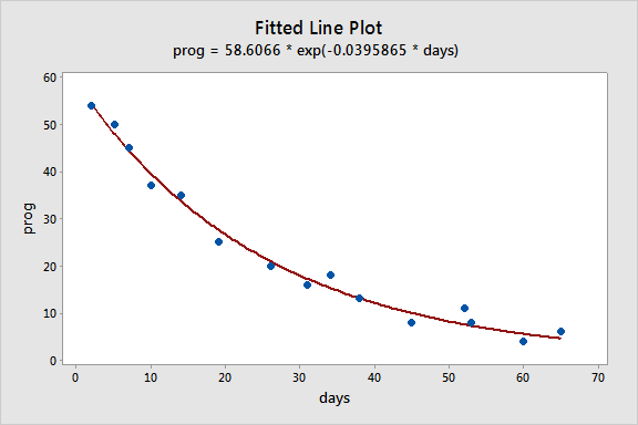
To illustrate, consider the example on long-term recovery after discharge from hospital from page 514 of Applied Linear Regression Models (4th ed) by Kutner, Nachtsheim, and Neter. The response variable, Y, is the prognostic index for long-term recovery and the predictor variable, X, is the number of days of hospitalization. The proposed model is the two-parameter exponential model:

\[\begin{equation*}
Y_{i}=\theta_{0}\exp(\theta_{1}X_i)+\epsilon_{i},
\end{equation*}\]

where the \(\epsilon_i\) are independent normal with constant variance.

Statistical software nonlinear regression routines are available to apply the Gauss-Newton algorithm to estimate \(\theta_0\) and \(\theta_1\). Before we do this, however, we have to find initial values for \(\theta_0\) and \(\theta_1\). One way to do this is to note that we can linearize the response function by taking the natural logarithm:

\[\begin{equation*}
\log(\theta_{0}\exp(\theta_{1}X_i)) = \log(\theta_{0}) + \theta_{1}X_i.
\end{equation*}\]

Thus we can fit a simple linear regression model with response, \(\log(Y)\), and predictor, \(X\), and the intercept (\(4.0372\)) gives us an estimate of \(\log(\theta_{0})\) while the slope (\(-0.03797\)) gives us an estimate of \(\theta_{1}\). (We then calculate \(\exp(4.0372)=56.7\) to estimate \(\theta_0\).)

Now we can fit the nonlinear regression model. The following output was obtained using Minitab:

Nonlinear Regression: prog = Theta1 * exp(Theta2 * days)

Method
Algorithm        Gauss-Newton
Max iterations            200
Tolerance             0.00001

Starting Values for Parameters
Parameter   Value
Theta1       56.7
Theta2     -0.038

Equation
prog = 58.6066 * exp(-0.0395865 * days)

Parameter Estimates
Parameter  Estimate  SE Estimate
Theta1      58.6066      1.47216
Theta2      -0.0396      0.00171

prog = Theta1 * exp(Theta2 * days)

Summary
Iterations        5
Final SSE   49.4593
DFE              13
MSE         3.80456
S           1.95053