The Poisson distribution for a random variable Y has the following probability mass function for a given value Y = y:

\[\begin{equation*}
\mbox{P}(Y=y|\lambda)=\frac{e^{-\lambda}\lambda^{y}}{y!},
\end{equation*}\]

for \(y=0,1,2,\ldots\). Notice that the Poisson distribution is characterized by the single parameter $\lambda$, which is the mean rate of occurrence for the event being measured. For the Poisson distribution, it is assumed that large counts (with respect to the value of $\lambda$) are rare.

In Poisson regression the dependent variable (Y) is an observed count that follows the Poisson distribution. The rate $\lambda$ is determined by a set of $k$  predictors $\textbf{X}=(X_{1},\ldots,X_{k})$. The expression relating these quantities is

\[\begin{equation*}
\lambda=\exp\{\textbf{X}\beta\}.
\end{equation*}\]

Thus, the fundamental Poisson regression model for observation i is given by

\[\begin{equation*}
\mbox{P}(Y_{i}=y_{i}|\textbf{X}_{i},\beta)=\frac{e^{-\exp\{\textbf{X}_{i}\beta\}}\exp\{\textbf{X}_{i}\beta\}^{y_{i}}}{y_{i}!}.
\end{equation*}\]

That is, for a given set of predictors, the categorical outcome follows a Poisson distribution with rate $\exp\{\textbf{X}\beta\}$. For a sample of size n, the likelihood for a Poisson regression is given by:

\[\begin{equation*}
L(\beta;\textbf{y},\textbf{X})=\prod_{i=1}^{n}\frac{e^{-\exp\{\textbf{X}_{i}\beta\}}\exp\{\textbf{X}_{i}\beta\}^{y_{i}}}{y_{i}!}.
\end{equation*}\]

This yields the log likelihood:

\[\begin{equation*}
\ell(\beta)=\sum_{i=1}^{n}y_{i}\textbf{X}_{i}\beta-\sum_{i=1}^{n}\exp\{\textbf{X}_{i}\beta\}-\sum_{i=1}^{n}\log(y_{i}!).
\end{equation*}\]

Maximizing the likelihood (or log likelihood) has no closed-form solution, so a technique like iteratively reweighted least squares is used to find an estimate of the regression coefficients, $\hat{\beta}$. Once this value of $\hat{\beta}$ has been obtained, we may proceed to define various goodness-of-fit measures and calculated residuals. For the residuals we present, they serve the same purpose as in linear regression. When plotted versus the response, they will help identify suspect data points.

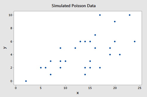
To illustrate consider this example (poisson_simulated.txt), which consists of a simulated data set of size n = 30 such that the response (Y) follows a Poisson distribution with rate $\lambda=\exp\{0.50+0.07X\}$. A plot of the response versus the predictor is given below. 

The following gives the analysis of the Poisson regression data:

Coefficients
Term        Coef  SE Coef       95% CI       Z-Value  P-Value   VIF
Constant   0.308    0.289  (-0.259,  0.875)     1.06    0.287
x         0.0764   0.0173  (0.0424, 0.1103)     4.41    0.000  1.00

Regression Equation
y  =  exp(Y')
Y' = 0.308 + 0.0764 x

As you can see, the Wald test p-value for x of 0.000 indicates that the predictor is highly significant.

Deviance Test

Changes in the deviance can be used to test the null hypothesis that any subset of the $\beta$'s is equal to 0. Suppose we test that r < k +1 of the $\beta$'s are equal to 0. Then the deviance test statistic is given by:

\[\begin{equation*}
G^2=-2\ell(\hat{\beta}^{(0)})-(-2\ell(\hat{\beta})),
\end{equation*}\]

where $-2\ell(\hat{\beta})$ is the deviance of the fitted (full) model and $-2\ell(\hat{\beta}^{(0)})$ is the deviance of the model specified by the null hypothesis evaluated at the maximum likelihood estimate of that reduced model. This test statistic has a $\chi^{2}$ distribution with \(k+1-r\) degrees of freedom. This test procedure is analagous to the general linear F test procedure for multiple linear regression.

To illustrate, the relevant software output from the simulated example is:

Deviance Table
Source      DF  Adj Dev  Adj Mean  Chi-Square  P-Value
Regression   1    20.47   20.4677       20.47    0.000
  x          1    20.47   20.4677       20.47    0.000
Error       28    27.84    0.9944
Total       29    48.31

Since there is only a single predictor for this example, this table simply provides information on the deviance test for x (p-value of 0.000), which matches the earlier Wald test result (p-value of 0.000). (Note that the Wald test and deviance test will not in general give identical results.) The Deviance Table includes the following:

• The null model in this case has no predictors, so the fitted values are simply the sample mean, \(4.233\). The deviance for the null model is \(-2\ell(\hat{\beta}^{(0)})=48.31\), which is shown in the "Total" row in the Deviance Table.
• The deviance for the fitted model is \(-2\ell(\hat{\beta})=27.84\), which is shown in the "Error" row in the Deviance Table.
• The deviance test statistic is therefore \(G^2=48.31-27.84=20.47\).
• The p-value comes from a $\chi^{2}$ distribution with \(2-1=1\) degrees of freedom.

Goodness-of-Fit

Overall performance of the fitted model can be measured by two different chi-square tests. There is the Pearson statistic

\[\begin{equation*}
X^2=\sum_{i=1}^{n}\frac{(y_{i}-\exp\{\textbf{X}_{i}\hat{\beta}\})^{2}}{\exp\{\textbf{X}_{i}\hat{\beta}\}}
\end{equation*}\]

and the deviance statistic

\[\begin{equation*}
D=2\sum_{i=1}^{n}\biggl[y_{i}\log\biggl(\frac{y_{i}}{\exp\{\textbf{X}_{i}\hat{\beta}\}}\biggr)-(y_{i}-\exp\{\textbf{X}_{i}\hat{\beta}\})\biggr].
\end{equation*}\]

Both of these statistics are approximately chi-square distributed with n – k – 1 degrees of freedom. When a test is rejected, there is a statistically significant lack of fit. Otherwise, there is no evidence of lack-of-fit.

To illustrate, the relevant software output from the simulated example is:

Goodness-of-Fit Tests
Test      DF  Estimate     Mean  Chi-Square  P-Value
Deviance  28  27.84209  0.99436       27.84    0.473
Pearson   28  26.09324  0.93190       26.09    0.568

The high p-values indicate no evidence of lack-of-fit.

Overdispersion means that the actual covariance matrix for the observed data exceeds that for the specified model for $Y|\textbf{X}$. For a Poisson distribution, the mean and the variance are equal. In practice, the data almost never reflects this fact and we have overdispersion in the Poisson regression model if (as is often the case) the variance is greater than the mean. In addition to testing goodness-of-fit, the Pearson statistic can also be used as a test of overdispersion. Note that overdispersion can also be measured in the logistic regression models that were discussed earlier.

Pseudo R²

The value of R² used in linear regression also does not extend to Poisson regression. One commonly used measure is the pseudo R², defined as

\[\begin{equation*}
R^{2}=\frac{\ell(\hat{\beta_{0}})-\ell(\hat{\beta})}{\ell(\hat{\beta_{0}})}=1-\frac{-2\ell(\hat{\beta})}{-2\ell(\hat{\beta_{0}})},
\end{equation*}\]

where $\ell(\hat{\beta_{0}})$ is the log likelihood of the model when only the intercept is included. The pseudo R² goes from 0 to 1 with 1 being a perfect fit.

To illustrate, the relevant software output from the simulated example is:

Model Summary
Deviance   Deviance
    R-Sq  R-Sq(adj)     AIC
  42.37%     40.30%  124.50

Recall from above that \(-2\ell(\hat{\beta})=27.84\) and \(-2\ell(\hat{\beta}^{(0)})=48.31\), so:

\[\begin{equation*}
R^{2}=1-\frac{27.84}{48.31}=0.4237.
\end{equation*}\]

Raw Residual

The raw residual is the difference between the actual response and the estimated value from the model. Remember that the variance is equal to the mean for a Poisson random variable. Therefore, we expect that the variances of the residuals are unequal. This can lead to difficulties in the interpretation of the raw residuals, yet it is still used. The formula for the raw residual is

\[\begin{equation*}
r_{i}=y_{i}-\exp\{\textbf{X}_{i}\beta\}.
\end{equation*}\]

Pearson Residual

The Pearson residual corrects for the unequal variance in the raw residuals by dividing by the standard deviation. The formula for the Pearson residuals is

\[\begin{equation*}
p_{i}=\frac{r_{i}}{\sqrt{\hat{\phi}\exp\{\textbf{X}_{i}\beta\}}},
\end{equation*}\]

where

\[\begin{equation*}
\hat{\phi}=\frac{1}{n-p}\sum_{i=1}^{n}\frac{(y_{i}-\exp\{\textbf{X}_{i}\hat{\beta}\})^{2}}{\exp\{\textbf{X}_{i}\hat{\beta}\}}.
\end{equation*}\]

$\hat{\phi}$ is a dispersion parameter to help control overdispersion.

Deviance Residuals

Deviance residuals are also popular because the sum of squares of these residuals is the deviance statistic. The formula for the deviance residual is

\[\begin{equation*}
d_{i}=\texttt{sgn}(y_{i}-\exp\{\textbf{X}_{i}\hat{\beta}\})\sqrt{2\biggl\{y_{i}\log\biggl(\frac{y_{i}}{\exp\{\textbf{X}_{i}\hat{\beta}\}}\biggr)-(y_{i}-\exp\{\textbf{X}_{i}\hat{\beta}\})\biggr\}}.
\end{equation*}\]

The plots below show the Pearson residuals and deviance residuals versus the fitted values for the simulated example.

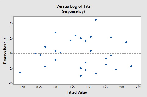
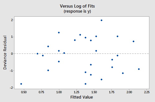
These plots appear to be good for a Poisson fit. Further diagnostic plots can also be produced and model selection techniques can be employed when faced with multiple predictors.

Hat Values

The hat matrix serves the same purpose as in the case of linear regression - to measure the influence of each observation on the overall fit of the model. The hat values, $h_{i,i}$, are the diagonal entries of the Hat matrix

\[\begin{equation*}
H=\textbf{W}^{1/2}\textbf{X}(\textbf{X}\textbf{W}\textbf{X})^{-1}\textbf{X}\textbf{W}^{1/2},
\end{equation*}\]

where W is an $n\times n$ diagonal matrix with the values of $\exp\{\textbf{X}_{i}\hat{\beta}\}$ on the diagonal. As before, a hat value (leverage) is large if $h_{i,i}>2p/n$.

Studentized Residuals

Finally, we can also report Studentized versions of some of the earlier residuals. The Studentized Pearson residuals are given by

\[\begin{equation*}
sp_{i}=\frac{p_{i}}{\sqrt{1-h_{i,i}}}
\end{equation*}\]

and the Studentized deviance residuals are given by

\[\begin{equation*}
sd_{i}=\frac{d_{i}}{\sqrt{1-h_{i, i}}}.
\end{equation*}\]

To illustrate, the relevant software output from the simulated example is:

Fits and Diagnostics for Unusual Observations
Obs       y    Fit  SE Fit       95% CI       Resid  Std Resid  Del Resid        HI  Cook’s D
  8  10.000  4.983   0.452  (4.171,  5.952)   1.974       2.02       2.03  0.040969      0.11
 21   6.000  8.503   1.408  (6.147, 11.763)  -0.907      -1.04      -1.02  0.233132      0.15
Obs      DFITS
  8   0.474408  R
 21  -0.540485     X
R  Large residual
X  Unusual X

The residuals in this output are deviance residuals, so observation 8 has a deviance residual of 1.974 and a studentized deviance residual of 2.02, while observation 21 has a leverage (h) of 0.233132.