Example 1: Toxicity Dataset

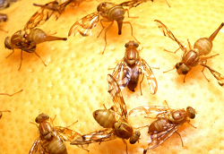
An experiment is done to test the effect of a toxic substance on insects. The data originate from the textbook, Applied Linear Statistical Models by Kutner, Nachtsheim, Neter, & Li.

At each of six dose levels, 250 insects are exposed to the substance and the number of insects that die is counted (toxicity.txt). We can use statistical software to calculate the observed probabilities as the number of observed deaths out of 250 for each dose level.

A binary logistic regression model is used to describe the connection between the observed probabilities of death as a function of dose level. The data is in event/trial format, which has to be taken into account by the statistical software used to conduct the analysis.

Software output is as follows:

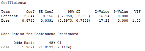
Thus

\[\hat{\pi}=\frac{\exp(-2.644+0.674X)}{1+\exp(-2.644+0.674X)}=\frac{1}{1+\exp(2.644-0.674X)}\]

where X = Dose and \(\hat{\pi}\) is the estimated probability the insect dies (based on the model).

Predicted probabilities of death (based on the logistic model) for the six dose levels are given below (FITS1). These probabilities closely agree with the observed values (Observed p) reported.

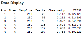
As an example of calculating the estimated probabilities, for Dose 1, we have

\[\hat{\pi}=\frac{1}{1+\exp(2.644-0.674(1))}=0.1224\]

The odds ratio for Dose is 1.9621, the value under Odds Ratio in the output. It was calculated as e^0.674. The interpretation of the odds ratio is that for every increase of 1 unit in dose level, the estimated odds of insect death are multiplied by 1.9621.

As an example of odds and odds ratio:

• At Dose = 1, the estimated odds of death is \(\hat{\pi}/(1− \hat{\pi})\) = 0.1224/(1−0.1224) = 0.1395.
• At Dose = 2, the estimated odds of death is \(\hat{\pi}/(1− \hat{\pi})\) = 0.2149/(1−0.2149) = 0.2737.
• The Odds Ratio = \(\frac{0.2737}{0.1395}=1.962\), which is the ratio of the odds of death when Dose = 2 compared to the odds when Dose = 1.

A property of the binary logistic regression model is that the odds ratio is the same for any increase of one unit in X, regardless of the specific values of X.

Example 2: STAT 200 Dataset

Students in STAT 200 at Penn State were asked if they have ever driven after drinking (dataset unfortunately no longer available). They also were asked, “How many days per month do you drink at least two beers?” In the following discussion, \(\pi\) = the probability a student says “yes” they have driven after drinking. This is modeled using X = days per month of drinking two beers. Results were as follows.

Some things to note from the results are:

• We see that in the sample 122/249 students said they have driven after drinking. (Yikes!)
• Parameter estimates, given under Coef are \(\hat{\beta}_0\) = −1.5514, and \(\hat{\beta}_1\) = 0.19031.
• The model for estimating \(\pi\) = the probability of ever having driven after drinking is

\[\hat{\pi}=\frac{\exp(-1.5514+0.19031X)}{1+\exp(-1.5514+0.19031X)}=\frac{1}{1+\exp(1.5514-0.19031X)}\]

• The variable X = DaysBeer is a statistically significant predictor (Z = 6.46, P = 0.000).

A plot of the estimated probability of ever having driven under the influence (\(\pi\)) versus days per month of drinking at least two beers is as follows:

The vertical axis shows the probability of ever having driven after drinking. For example, if X = 4 days per month of drinking beer, then the estimated probability is calculated as:

\[\hat{\pi}=\frac{1}{1+\exp(1.5514-0.19031(4))}=\frac{1}{1+\exp(0.79016)}=0.312\]

A few of these estimated probabilities are given in the following table:

In the results given above, we see that the estimate of the odds ratio is 1.21 for DaysBeer. This is given under Odds Ratio in the table of coefficients, standard errors and so on. The sample odds ratio was calculated as e^0.19031. The interpretation of the odds ratio is that for each increase of one day of drinking beer per month, the predicted odds of having ever driven after drinking are multiplied by 1.21.

Above we found that at X = 4, the predicted probability of ever driving after drinking is \(\hat{\pi}\) = 0.312. Thus when X = 4, the predicted odds of ever driving after drinking is 0.312/(1 − 0.312) = 0.453. To find the odds when X = 5, one method would be to multiply the odds at X = 4 by the sample odds ratio. The calculation is 1.21 × 0.453 = 0.549. (Another method is to just do the calculation using the predicted probability at X = 5, as we did above for X = 4.)

Notice also, that the results give a 95% confidence interval estimate of the odd ratio (1.14 to 1.28).

We now include Gender (male or female) as an x-variable (along with DaysBeer). Some results are given below. Under Gender, the row for male corresponds to an indicator variable with a value of 1 if the student is male and a value of 0 if the student is female.

Some things to note from the results are:

• The p-values are less than 0.05 for both DaysBeer and Gender. This is evidence that both x-variables are useful for predicting the probability of ever having driven after drinking.
• For DaysBeer, the odds ratio is still estimated to equal 1.21 to two decimal places (calculated as e^0.18693).
• For Gender, the odds ratio is 1.85 (calculated as  e^0.6172). For males, the odds of ever having driven after drinking is 1.85 times the odds for females, assuming DaysBeer is held constant.

Finally, the results for testing with respect to the multiple logistic regression model are as follows:

Notice that since we have a p-value of 0.000 for this chi-square test, we therefore reject the null hypothesis that all of the slopes are equal to 0.