12.7 - Population Growth Example
 Census Data
A simple model for population growth towards an asymptote is the logistic model
\[\begin{equation*}
y_{i}=\frac{\beta_{1}}{1+\exp(\beta_{2}+\beta_{3}x_{i})}+\epsilon_{i},
\end{equation*}\]
where $y_{i}$ is the population size at time $x_{i}$, $\beta_{1}$ is the asymptote towards which the population grows, $\beta_{2}$ reflects the size of the population at time x = 0 (relative to its asymptotic size), and $\beta_{3}$ controls the growth rate of the population.
We fit this model to Census population data (us_census.txt) for the United States (in millions) ranging from 1790 through 1990 (see below).
| year | population |
| 1790 | 3.929 |
| 1800 | 5.308 |
| 1810 | 7.240 |
| 1820 | 9.638 |
| 1830 | 12.866 |
| 1840 | 17.069 |
| 1850 | 23.192 |
| 1860 | 31.443 |
| 1870 | 39.818 |
| 1880 | 50.156 |
| 1890 | 62.948 |
| 1900 | 75.995 |
| 1910 | 91.972 |
| 1920 | 105.711 |
| 1930 | 122.775 |
| 1940 | 131.669 |
| 1950 | 150.697 |
| 1960 | 179.323 |
| 1970 | 203.302 |
| 1980 | 226.542 |
| 1990 | 248.710 |
The data are graphed (see below) and the line represents the fit of the logistic population growth model.
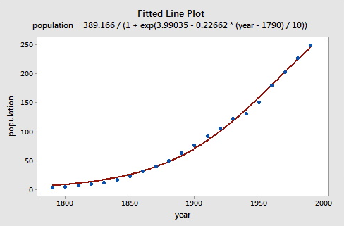
To fit the logistic model to the U. S. Census data, we need starting values for the parameters. It is often important in nonlinear least squares estimation to choose reasonable starting values, which generally requires some insight into the structure of the model. We know that $\beta_{1}$ represents asymptotic population. The data in the plot above show that in 1990 the U. S. population stood at about 250 million and did not appear to be close to an asymptote; so as not to extrapolate too far beyond the data, let us set the starting value of $\beta_{1}$ to 350. It is convenient to scale time so that $x_{1}=0$ in 1790, and so that the unit of time is 10 years.
Then substituting $\beta_{1}=350$ and $x=0$ into the model, using the value $y_{1}=3.929$ from the data, and assuming that the error is 0, we have
\[\begin{equation*}
3.929=\frac{350}{1+\exp(\beta_{2}+\beta_{3}(0))}.
\end{equation*}\]
Solving for $\beta_{2}$ gives us a plausible start value for this parameter:
\[\begin{align*}
\exp(\beta_{2})&=\frac{350}{3.929}-1\\
\beta_{2}&=\log\biggl(\frac{350}{3.929}-1\biggr)\approx 4.5.
\end{align*}\]
Finally, returning to the data, at time x = 1 (i.e., at the second Census performed in 1800), the population was $y_{2}=5.308$. Using this value, along with the previously determined start values for $\beta_{1}$ and $\beta_{2}$, and again setting the error to 0, we have
\[\begin{equation*}
5.308=\frac{350}{1+\exp(4.5+\beta_{3}(1))}.
\end{equation*}\]
Solving for $\beta_{3}$ we get
\[\begin{align*}
\exp(4.5+\beta_{3})&=\frac{350}{5.308}-1\\
\beta_{3}&=\log\biggl(\frac{350}{5.308}-1\biggr)-4.5\approx -0.3.
\end{align*}\]
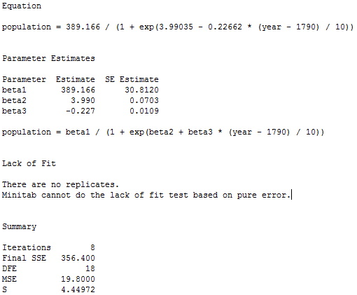
So now we have starting values for the nonlinear least squares algorithm that we use. Below is the output from fitting the model in Minitab using Gauss-Netwon.
As you can see, the starting values resulted in convergence with values not too far from our guess.
Here is a plot of the residuals versus the year.
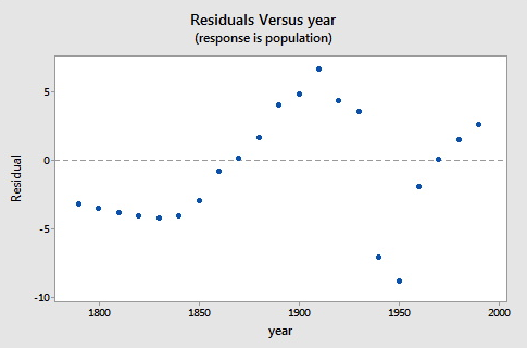
As the earlier fitted line plot showed, the logistic functional form that we chose did catch the gross characteristics of this data. However, as the above residual plot shows, some of the nuances appear to not be as well characterized. Since there are indications of some cyclical behavior, a model incorporating correlated errors or, perhaps, trigonometric functions could be investigated.

