If the two models have nearly the same values for the odds ratio, choose the simpler one.
However, what is ”nearly the same values”? What do we do?
This is a subjective decision, and depends on the purpose of the data.
|
Fitted Odds Ratio
|
||||
|
Model
|
W - S
|
M - W
|
M - S
|
|
| (MS, MW) |
1.00
|
2.40
|
4.32
|
|
| (MS, WS, MW) |
1.47
|
2.11
|
4.04
|
|
| Observed or | (MSW) - level 1 |
1.55
|
2.19
|
4.26
|
| (MSW) - level 2 |
1.42
|
2.00
|
3.90
|
|
They seem close enough, but what else can we look at...
Dissimilarity Index
The Dissimilarity Index is a summary statistic describing how close the fitted values of a model are to the observed data (e.g. observed counts). For a table of any dimension, it equals
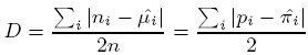
For our example used in this lesson, see collarDIndex.sas.
For the model (MW, MS):
D = 55.2306 / 2 (715) = 0.039
What does this mean? We could interpret this values such that, we would need to move 3.9% percent of the observations to achieve a perfect fit of the model (MW, MS) to observed (sample) data.
For the model (MW, MS, SW):
D = 5.8888 / 2 (715) = 0.004
Here we would only need to move 0.4% of the observations to achieve a perfect fit of the models (MW, MS, SW) to the observed data.
Which one do we use? Possibly the model of conditional independence. I, personally, could be OK with moving about 3.9% of the data.
Properties of D
- 0 ≤ D ≤ 1
- D = the proportion of sample cases that need to move to a different cell to have the model fit perfectly.
- Small D means that there is little difference between fitted values and observed counts.
- Larger D means that there is a big difference between fitted values and observed counts.
- D is an estimate of the change, Δ, which measures the lack-of-fit of the model in the population.
- When the model fits perfectly in the population: Δ = 0, and D overestimates the lack-of-fit (especially for small samples).
- For large samples when the model does not fit perfectly: G2 > and X2 will be large, and D reveals when the lack-of-fit is important in a practical sense.
- Rule-of-thumb: D < 0.03 indicates non-important lack-of-fit.
Correlations between observed and fitted counts
A large correlation value indicates that the observed and fitted values are close.
For our example, for the conditional independence model (MW, MS) in our example, r = 0.9906, and for the homogeneous model, r = 0.9999. Is there really a difference here? If I round to two decimal places, there is no difference at all!
Information Criteria
These are different statistics that compare fitted and observed values, that is the loglikelihoods of two models, but take into account the complexity of the model and/or sample size.
The complexity typically refers to the number of parameters in the model.
Note: Unlike partial association tests, these statistics do NOT require the models to be nested.
The two most commonly used ones are:
Akiake Information Criteria (AIC)
AIC = −2 × LogL + 2 × number of parameters
Bayesian Information Criteria (BIC)
BIC = G2 − (df) × logN = −2 × log(B)
where N = total number of observations, and B = posterior odds.
Note: The smaller the value, the better the model.
BIC Statistic and Bayesian Model Selection
BIC gives a way of considering the trade-off between a simple parsimonous model (practical significance) and a more complex and closer to reality model (statistical significance).
Suppose we are considering a model M0, and comparing it to the saturated model, M1. Which model gives a better description of the main features as reflected in the data? (e.g. which of the two is more likely to be the true model? We can use posterior odds which then figure into the BIC:
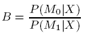
where X = data.
- When comparing a set of models, choose the one with the smallest BIC value.
- If BIC is negative choose M0
- The models do not have to be nested.
- This procedure provides you with a consistent model in the sense that in large samples, it chooses the correct model with high probability.
The following table gives both BIC and AIC for our running example.
|
Model
|
df
|
G2
|
p-value
|
BIC
|
Parameters
|
AIC
|
| (MSW) |
0
|
0.00
|
1.000
|
.00
|
8
|
-
|
| (MS)(MW)(SW) |
1
|
.06
|
.800
|
-6.51
|
7
|
-13.94
|
| (MW)(SW) |
2
|
71.90
|
.000
|
58.76
|
6
|
59.90
|
| (MS)(WS) |
2
|
19.71
|
.000
|
6.57
|
6
|
7.71
|
| (SM)(WM) |
2
|
5.39
|
.068
|
-7.75
|
6
|
-6.61
|
| (MW)(S) |
3
|
87.79
|
.000
|
68.07
|
5
|
77.79
|
| (WS)(M) |
3
|
102.11
|
.000
|
82.07
|
5
|
92.11
|
| (MS)(W) |
3
|
35.60
|
.000
|
15.88
|
5
|
25.60
|
| (M)(S)(W) |
4
|
118.00
|
.000
|
91.71
|
4
|
110.00
|

Which model would you choose based on BIC? How about AIC? Is it the same model?
Look for the smallest value. In this case the smallest BIC is -7.75, indicating the conditional independence model. How about AIC?
Please note that there is a lot of debate about which value, BIC or AIC is more helpful. Best is to report both when making your decision.
References:
- Raftery, A.E. (1985). A note on Bayes factors for log-linear contingency table models with vague prior information. Journal of the Royal Statistical Society, Series B.
- Raftery, A. E. (1986). Choosing models for cross-classifications. American Sociological Review, 51, 145146.
- Spiegelhalter, D.J. and Smith, A.F.M. (1982). Bayes Factors for linear and log-linear models with vague prior information. Journal of the Royal Statistical Society, Series B, 44, 377387.