3 Identifying and Estimating ARIMA models; Using ARIMA models to forecast future values
ARIMA
Statistical significance
Forecasting
R Code
Overview
In this lesson, we will learn some techniques for identifying and estimating non-seasonal ARIMA models. We’ll also look at the basics of using an ARIMA model to make forecasts. We’ll look at seasonal ARIMA models next week. Lesson 3.1 gives the basic ideas for determining a model and analyzing residuals after a model has been estimated. Lesson 3.2 gives a test for residual autocorrelations. Lesson 3.3 gives some basics for forecasting using ARIMA models. We’ll look at other forecasting models later in the course. This all relates to Chapter 3 in the book, although the authors give quite a theoretical treatment of the topic(s).
Objectives
Upon completion of this lesson, you should be able to:
- Identify and interpret a non-seasonal ARIMA model
- Distinguish ARIMA terms from simultaneously exploring an ACF and PACF.
- Test that all residual autocorrelations are zero.
- Convert ARIMA models to infinite order MA models.
- Forecast with ARIMA models.
- Create and interpret prediction intervals for forecasts.
3.1 Non-seasonal ARIMA Models
ARIMA models, also called Box-Jenkins models, are models that may possibly include autoregressive terms, moving average terms, and differencing operations. Various abbreviations are used:
- When a model only involves autoregressive terms it may be referred to as an AR model. When a model only involves moving average terms, it may be referred to as an MA model.
- When no differencing is involved, the abbreviation ARMA may be used.
Specifying the Elements of the Model
In most software programs, the elements in the model are specified in the order (AR order, differencing, MA order). As examples,
A model with (only) two AR terms would be specified as an ARIMA of order (2,0,0).
A MA(2) model would be specified as an ARIMA of order (0,0,2).
A model with one AR term, a first difference, and one MA term would have order (1,1,1).
For the last model, ARIMA (1,1,1), a model with one AR term and one MA term is being applied to the variable \(Z_{t}=X_{t}-X_{t-1}.\) A first difference might be used to account for a linear trend in the data.
The differencing order refers to successive first differences. For example, for a difference order = 2 the variable analyzed is \(z_{t}=\left(x_{t}-x_{t-1}\right)-\left(x_{t-1}-x_{t-2}\right),\) the first difference of first differences. This type of difference might account for a quadratic trend in the data.
Identifying a Possible Model
Three items should be considered to determine the first guess at an ARIMA model: a time series plot of the data, the ACF, and the PACF.
Time series plot of the observed series
In Lesson 1.1, we discussed what to look for: possible trend, seasonality, outliers, constant variance or nonconstant variance.
- You won’t be able to spot any particular model by looking at this plot, but you will be able to see the need for various possible actions.
- If there’s an obvious upward or downward linear trend, a first difference may be needed. A quadratic trend might need a 2nd order difference (as described above). We rarely want to go much beyond two. In those cases, we might want to think about things like smoothing, which we will cover later in the course. Over-differencing can cause us to introduce unnecessary levels of dependency (difference white noise to obtain an MA(1)–difference again to obtain an MA(2), etc.)
- For data with a curved upward trend accompanied by increasing variance, you should consider transforming the series with either a logarithm or a square root.
ACF and PACF
The ACF and PACF should be considered together. It can sometimes be tricky going, but a few combined patterns do stand out. Note that each pattern includes a discussion of both plots and so you should always describe how both plots suggest a model.(These are listed in Table 3.1 of the book in Section 3.3).
AR models have theoretical PACFs with non-zero values at the AR terms in the model and zero values elsewhere. The ACF will taper to zero in some fashion.
An AR(1) model has a single spike in the PACF and an ACF with a pattern
\[\rho_k = \phi_1^k\]
An AR(2) has two spikes in the PACF and a sinusoidal ACF that converges to 0.
MA models have theoretical ACFs with non-zero values at the MA terms in the model and zero values elsewhere. The PACF will taper to zero in some fashion.
ARMA models (including both AR and MA terms) have ACFs and PACFs that both tail off to 0. These are the trickiest because the order will not be particularly obvious. Basically, you just have to guess that one or two terms of each type may be needed and then see what happens when you estimate the model.
If the ACF does not tail off, but instead has values that stay close to 1 over many lags, the series is non-stationary and differencing will be needed. Try a first difference and then look at the ACF and PACF of the differenced data.
If the series autocorrelations are non-significant, then the series is random (white noise; the ordering matters, but the data are independent and identically distributed.) You’re done at that point.
If first differences were necessary and all the differenced autocorrelations are non-significant, then the original series is called a random walk and you are done. (A possible model for a random walk is \(x_t=\delta+x_{t-1}+w_t.\) The data are dependent and are not identically distributed; in fact both the mean and variance are increasing through time.)
Estimating and Diagnosing a Possible Model
After you’ve made a guess (or two) at a possible model, use software such as R, Minitab, or SAS to estimate the coefficients. Most software will use maximum likelihood estimation methods to make the estimates. Once the model has been estimated, do the following.
- Look at the significance of the coefficients. In R,
sarimaprovides p-values and so you may simply compare the p-value to the standard 0.05 cut-off. Thearimacommand does not provide p-values and so you can calculate a t-statistic: \(t\) = estimated coeff. / std. error of coeff. Recall that \(t_{\alpha,df}\) is the Student \(t\)-value with area \(\alpha\) to the right of \(t_{\alpha,df}\) on df degrees of freedom. If \(\lvert t \rvert>t_{0.025,n-p-q-1},\) then the estimated coefficient is significantly different from 0. When n is large, you may compare estimated coeff. / std. error to 1.96. - Look at the ACF of the residuals. For a good model, all autocorrelations for the residual series should be non-significant. If this isn’t the case, you need to try a different model.
- Look at Box-Pierce (Ljung) tests for possible residual autocorrelation at various lags (see Lesson 3.2 for a description of this test).
- If non-constant variance is a concern, look at a plot of residuals versus fits and/or a time series plot of the residuals.
If something looks wrong, you’ll have to revise your guess at what the model might be. This might involve adding parameters or re-interpreting the original ACF and PACF to possibly move in a different direction.
What if More Than One Model Looks Okay?
Sometimes more than one model can seem to work for the same dataset. When that’s the case, some things you can do to decide between the models are:
- Possibly choose the model with the fewest parameters.
- Examine standard errors of forecast values. Pick the model with the generally lowest standard errors for predictions of the future.
- Compare models with regard to statistics such as the MSE (the estimate of the variance of the \(w_t\)), AIC, AICc, and SIC (also called BIC). Lower values of these statistics are desirable.
AIC, AICc, and SIC (or BIC) are defined and discussed in Section 2.1 of our text. The statistics combine the estimate of the variance with values of the sample size and number of parameters in the model.
One reason that two models may seem to give about the same results is that, with the certain coefficient values, two different models can sometimes be nearly equivalent when they are each converted to an infinite order MA model. [Every ARIMA model can be converted to an infinite order MA – this is useful for some theoretical work, including the determination of standard errors for forecast errors.] We’ll see more about this in Lesson 3.2.
Example 3.1 (Lake Erie) The Lake Erie data (eriedata.dat) from Week 1 assignment. The series is n = 40 consecutive annual measurements of the level of Lake Erie in October.
Identifying the model
A time series plot of the data is the following:
Show the R code
# Load the data from eriedata.dat
xerie = scan("data_files/eriedata.dat") #reads the data
xerie = ts (xerie) # makes sure xerie is a time series object
plot (xerie, type = "b") # plots xerie

# We first loaded the astsa library discussed in Lesson 1. It’s a set of scripts written by Stoffer, one of the textbook’s authors. If you installed the astsa package during Lesson 1, then you only need the library command.

# Use the command library("astsa"). This makes the downloaded routines accessible.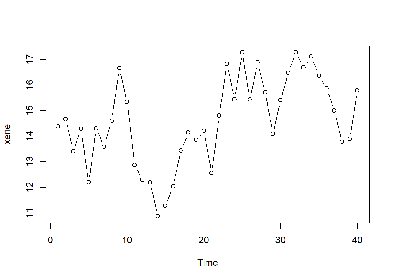
There’s a possibility of some overall trend, but it might look that way just because there seemed to be a big dip around the 15th time or so. We’ll go ahead without worrying about trend.
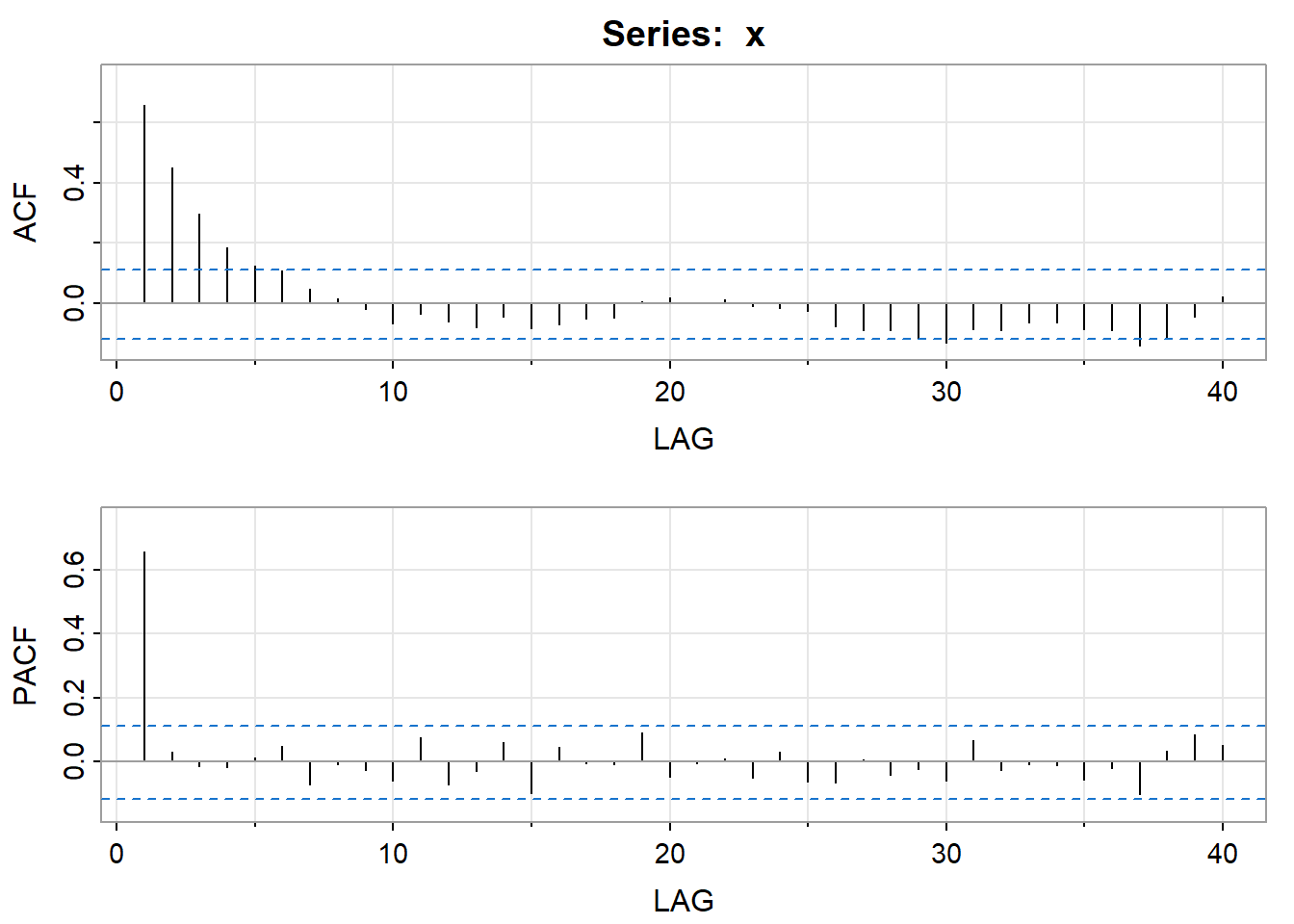
The ACF and the PACF of the series are the following. (They start at lag 1).
Show the R code
acf2 (xerie) # author’s routine for graphing both the ACF and the PACF [,1] [,2] [,3] [,4] [,5] [,6] [,7] [,8] [,9]
ACF 0.7 0.54 0.36 0.21 0.17 0.12 0.18 0.20 0.16
PACF 0.7 0.10 -0.09 -0.08 0.11 -0.01 0.18 0.02 -0.09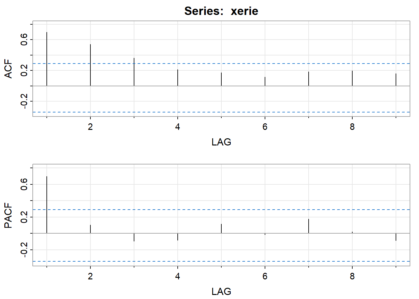
The PACF shows a single spike at the first lag and the ACF shows a tapering pattern. An AR(1) model is indicated.
Estimating the Model
We used the R script sarima, written by one of the authors of our book (Stoffer), to estimate the AR(1) model. Here’s part of the output:
Show the R code
sarima (xerie, 1, 0, 0, details = FALSE) # this is the AR(1) model estimated with the author’s routine<><><><><><><><><><><><><><>
Coefficients:
Estimate SE t.value p.value
ar1 0.6909 0.1094 6.3126 0
xmean 14.6309 0.5840 25.0523 0
sigma^2 estimated as 1.446814 on 38 degrees of freedom
AIC = 3.373462 AICc = 3.38157 BIC = 3.500128
Where the coefficients are listed, notice the heading “xmean.” This is giving the estimated mean of the series based on this model, not the intercept. The model used in the software is of the form \((x_t - \mu) = \phi_1(x_{t-1}-\mu)+w_t.\)
The estimated model can be written as \[(x_t - 14.6309) = 0.6909(x_{t-1} - 14.6309) + w_t.\]
This is equivalent to \[\begin{align}x_t &= 14.6309 - (14.6309*0.6909) + 0.6909x_{t-1} + w_t\\ &= 4.522 + 0.6909x_{t-1} + w_t\end{align}.\]
The AR coefficient is statistically significant \((z = 0.6909/0.1094 = 6.315).\) It’s not necessary to test the mean coefficient. We know that it’s not 0.
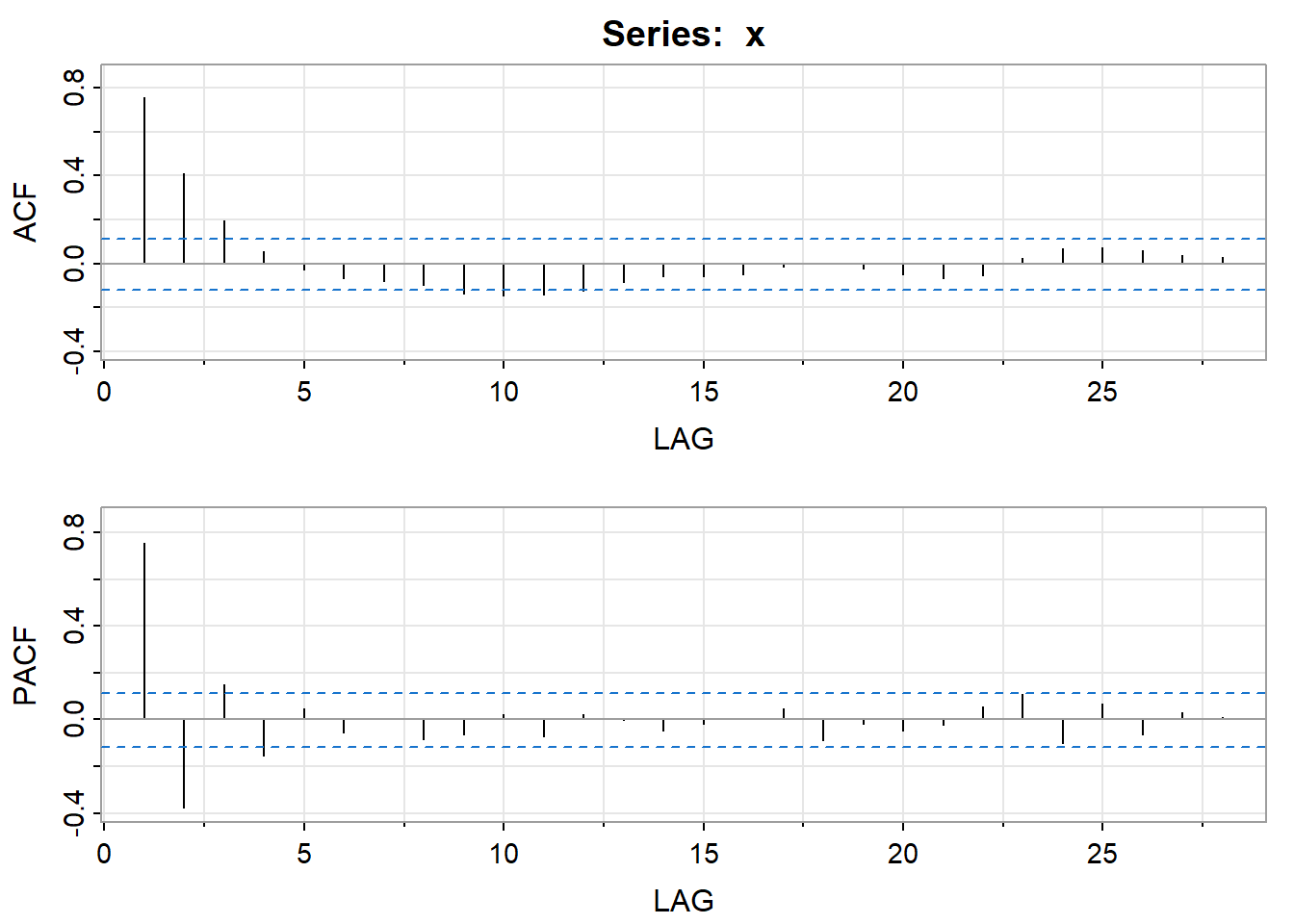
The author’s routine also gives residual diagnostics in the form of several graphs. Here’s that part of the output:
Show the R code
sarima (xerie, 1, 0, 0) # this is the AR(1) model estimated with the author’s routine
Interpretations of the Diagnostics
The time series plot of the standardized residuals mostly indicates that there’s no trend in the residuals, no outliers, and in general, no changing variance across time.
The ACF of the residuals shows no significant autocorrelations – a good result.
The Q-Q plot is a normal probability plot. It doesn’t look too bad, so the assumption of normally distributed residuals looks okay.
The bottom plot gives p-values for the Ljung-Box-Pierce statistics for each lag up to 20. These statistics consider the accumulated residual autocorrelation from lag 1 up to and including the lag on the horizontal axis. The dashed blue line is at .05. All p-values are above it. That’s a good result. We want non-significant values for this statistic when looking at residuals. Read Lesson 3.2 of this week for more about the Ljung–Box-Pierce statistic.
All in all, the fit looks good. There’s not much need to continue, but just to show you how things look when incorrect models are used, we will present another model.
Output for a Wrong Model
Suppose that we had misinterpreted the ACF and PACF of the data and had tried an MA(1) model rather than the AR(1) model.
Here’s the output:
Show the R code
sarima (xerie, 0, 0, 1, details = FALSE) # this is the incorrect MA(1) model<><><><><><><><><><><><><><>
Coefficients:
Estimate SE t.value p.value
ma1 0.5570 0.1251 4.4530 1e-04
xmean 14.5881 0.3337 43.7213 0e+00
sigma^2 estimated as 1.869631 on 38 degrees of freedom
AIC = 3.622905 AICc = 3.631013 BIC = 3.74957
The MA(1) coefficient is significant (you can check it), but mostly this looks worse than the statistics for the right model. The estimate of the variance is 1.87, compared to 1.447 for the AR(1) model. The AIC and BIC statistics are higher for the MA(1) than for the AR(1). That’s not good.
The diagnostic graphs aren’t good for the MA(1). The ACF has a significant spike at lag 2 and several of the Ljung-Box-Pierce p-values are below .05. We don’t want them there. So, the MA(1) isn’t a good model.
Show the R code
sarima (xerie, 0, 0, 1) # this is the incorrect MA(1) model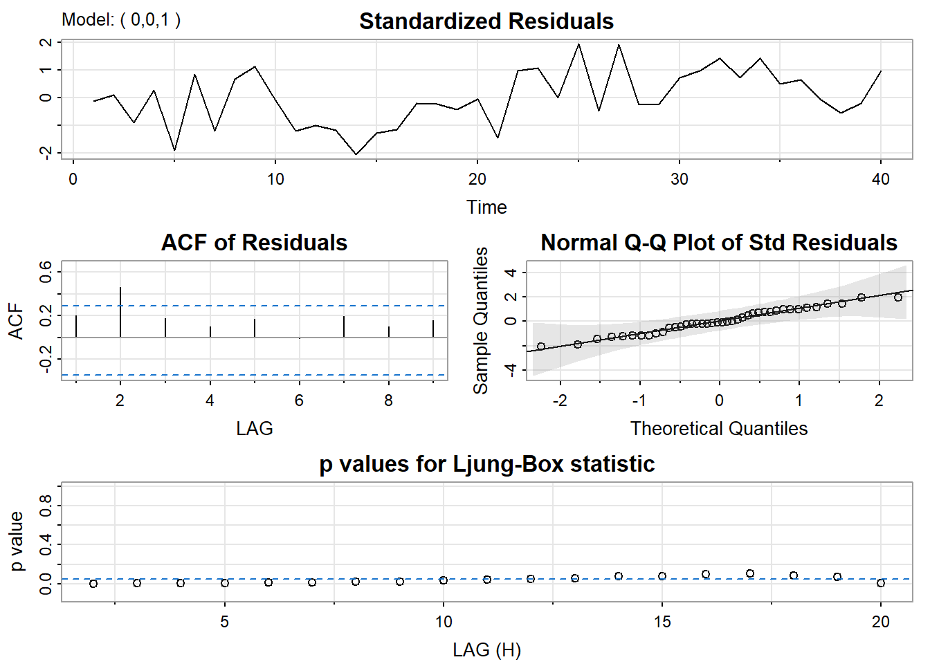
A Model with One Too Many Coefficients
Suppose we try a model (still the Lake Erie Data) with one AR term and one MA term. Here’s some of the output:
Show the R code
sarima (xerie, 1, 0, 1, details = FALSE) # this is the over-parameterized ARMA(1,1) model <><><><><><><><><><><><><><>
Coefficients:
Estimate SE t.value p.value
ar1 0.7362 0.1362 5.4073 0.0000
ma1 -0.0909 0.1969 -0.4614 0.6472
xmean 14.6307 0.6142 23.8196 0.0000
sigma^2 estimated as 1.439188 on 37 degrees of freedom
AIC = 3.418224 AICc = 3.434891 BIC = 3.587112
Example 3.2 (Parameter Redundancy) Suppose that the model for your data is white noise. If this is true for every \(t,\) then it is true for \(t-1\) as well, in other words:
\[x_t = w_t\]
\[x_{t-1} = w_{t-1}\]
Let’s multiply both sides of the second equation by 0.5:
\[0.5x_{t-1} = 0.5w_{t-1}\]
Next, we will move both terms over to one side:
\[0 = -0.5x_{t-1} + 0.5w_{t-1}\]
Because the data is white noise, \(x_t=w_t,\) so we can add \(x_t\) to the left side and \(w_t\) to the right side:
\[x_t = -0.5x_{t-1} + w_t + 0.5w_{t-1}\]
This is an ARMA(1, 1)! The problem is that we know it is white noise because of the original equations. If we looked at the ACF what would we see? You would see the ACF corresponding to white noise, a spike at zero and then nothing else. This also means if we take the white noise process and you try to fit in an ARMA(1, 1), R will do it and will come up with coefficients that look something like what we have above. This is one of the reasons why we need to look at the ACF and the PACF plots and other diagnostics. We prefer a model with the fewest parameters. This example also says that for certain parameter values, ARMA models can appear very similar to one another.
R-Code for Example 3.1
Here’s how we accomplished the work for the example in this lesson.
We first loaded the astsa library discussed in Lesson 1. It’s a set of scripts written by Stoffer, one of the textbook’s authors. If you installed the astsa package during Lesson 1, then you only need the library command.
Use the command library(astsa). This makes the downloaded routines accessible.
The session for creating Example 1 then proceeds as follows:
xerie = scan("eriedata.dat") #reads the data
xerie = ts (xerie) # makes sure xerie is a time series object
plot (xerie, type = "b") # plots xerie
acf2 (xerie) # author’s routine for graphing both the ACF and the PACF
sarima (xerie, 1, 0, 0) # this is the AR(1) model estimated with the author’s routine
sarima (xerie, 0, 0, 1) # this is the incorrect MA(1) model
sarima (xerie, 1, 0, 1) # this is the over-parameterized ARMA(1,1) model
In Lesson 3.3, we’ll discuss the use of ARIMA models for forecasting. Here’s how you would forecast for the next 4 times past the end of the series using the author’s source code and the AR(1) model for the Lake Erie data.
sarima.for(xerie, 4, 1, 0, 0) # four forecasts from an AR(1) model for the erie data You’ll get forecasts for the next four times, the standard errors for these forecasts, and a graph of the time series along with the forecasts. More details about forecasting will be given in Lesson 3.3.
Some useful information about the author’s scripts are available at the Time Series Analysis and Its Applications online resources.
3.2 Diagnostics
Analyzing possible statistical significance of autocorrelation values
The Ljung-Box statistic, also called the modified Box-Pierce statistic, is a function of the accumulated sample autocorrelations, \(r_j,\) up to any specified time lag \(m.\) As a function of \(m,\) it is determined as:
\[Q(m) = n(n+2)\sum_{j=1}^{m}\frac{r^2_j}{n-j},\]
where n = number of usable data points after any differencing operations. (Please visit forvo for the proper pronunciation of Ljung.)
As an example,
\[Q(3) = n(n+2)\left(\frac{r^2_1}{n-1}+\frac{r^2_2}{n-2}+\frac{r^2_3}{n-3}\right)\]
Use of the Statistic
This statistic can be used to examine residuals from a time series model in order to see if all underlying population autocorrelations for the errors may be 0 (up to a specified point).
For nearly all models that we consider in this course, the residuals are assumed to be “white noise,” meaning that they are identically, independently distributed (from each other). Thus, as we saw last week, the ideal ACF for residuals is that all autocorrelations are 0. This means that \(Q(m)\) should be 0 for any lag \(m.\) A significant \(Q(m)\) for residuals indicates a possible problem with the model.
(Remember \(Q(m)\) measures accumulated autocorrelation up to lag \(m.\))
Distribution of \(Q(m)\)
There are two cases:
- When the \(r_j\) are sample autocorrelations for residuals from a time series model, the null hypothesis distribution of \(Q(m)\) is approximately a \(\chi^2\) distribution with df = \(m-p-q-1,\) where \(p+q+1\) is the number of coefficients in the model, including a constant.
- When no model has been used, so that the ACF is for raw data, the null distribution of \(Q(m)\) is
approximately a \(\chi^2\) distribution with df = \(m.\)
p-Value Determination
In both cases, a p-value is calculated as the probability past \(Q(m)\) in the relevant distribution. A small p-value (for instance, p-value < .05) indicates the possibility of non-zero autocorrelation within the first \(m\) lags.
Example 3.3 Below there is Minitab output for the Lake Erie level data that was used for homework 1 and in Lesson 3.1. A useful model is an AR(1) with a constant. So \(p+q+1=1+0+1=2.\)
Final Estimates of Parameters
| Type | Coef | SE Coef | T-Value | P-Value |
|---|---|---|---|---|
| AR 1 | 0.708 | 0.116 | 6.10 | 0.000 |
| Constant | 4.276 | 0.195 | 21.89 | 0.000 |
| Mean | 14.635 | 0.668 |
Modified Box-Pierce (Ljung-Box) Chi-Square statistic
| Lag | 12 | 24 | 36 | 48 |
|---|---|---|---|---|
| Chi-Square | 9.42 | 23.21 | 30.05 | * |
| DF | 10 | 22 | 34 | * |
| P-Value | 0.493 | 0.390 | 0.662 | * |
Minitab gives p-values for accumulated lags that are multiples of 12. The R sarima command will give a graph that shows p-values of the Ljung-Box-Pierce tests for each lag (in steps of 1) up to a certain lag, usually up to lag 20 for nonseasonal models.
Interpretation of the Box-Pierce Results
Notice that the p-values for the modified Box-Pierce all are well above .05, indicating “non-significance.” This is a desirable result. Remember that there are only 40 data values, so there’s not much data contributing to correlations at high lags. Thus, the results for and may not be meaningful for these data.
Graphs of ACF values
When you request a graph of the ACF values, “significance” limits are shown by R and by Minitab. In general, the limits for the autocorrelation are placed at \(0 ± 2\) standard errors of \(r_k.\) The formula used for standard error depends upon the situation.
- Within the ACF of residuals as part of the ARIMA routine, the standard errors are determined assuming the residuals are white noise. The approximate formula for any lag is that s.e. of \(r_k=1/\sqrt{n}.\)
- For the ACF of raw data (the ACF command), the standard error at a lag k is found as if the right model was an MA(k-1). This allows the possible interpretation that if all autocorrelations past a certain lag are within the limits, the model might be an MA of order defined by the last significant autocorrelation.
Appendix: Standardized Residuals
What are standardized residuals in a time series framework? One of the things that we need to look at when we look at the diagnostics from a regression fit is a graph of the standardized residuals. Let’s review what this is for regular regression where the standard deviation is \(\sigma.\) The standardized residual at observation i
\[\dfrac{y_i - \beta_0 - \sum_{j=1}^{p}\beta_j x_{ij}}{\sigma},\]
should be \(N(0, 1).\) We hope to see normality when we look at the diagnostic plots. Another way to think about this is:
\[\dfrac{y_i - \beta_0 -\sum_{j=1}^{p}\beta_j x_{ij}}{\sigma} \approx \dfrac{y_i - \widehat{y}_i}{\sqrt{Var(y_i - \widehat{y}_i)}}.\]
Now, with time series things are very similar:
\[\dfrac{x_t-\tilde{x_t}}{\sqrt{P^{t-1}_t}},\]
where
\[\tilde{x_t} = E(x_t|x_{t-1}, x_{t-2}, \dots) \text{ and } P^{t-1}_t = E\left[(x_t-\tilde{x_t})^2\right].\]
This is where the standardized residuals come from. This is also essentially how a time series is fit using R. We want to minimize the sums of these squared values:
\[\sum_{t=1}^{n}\left(\dfrac{x_t - \tilde{x_t}}{\sqrt{P^{t-1}_t}}\right)^2\]
(In reality, it is slightly more complicated. The log-likelihood function is minimized, and this is one term of that function.)
3.3 Forecasting with ARIMA Models
Section 3.4 in the textbook gives a theoretical look at forecasting with ARIMA models. That presentation is a bit tough, but in practice, it’s easy to understand how forecasts are created.
In an ARIMA model, we express \(x_t\) as a function of past value(s) of x and/or past errors (as well as a present time error). When we forecast a value past the end of the series, we might need values from the observed series on the right side of the equation or we might, in theory, need values that aren’t yet observed.
Example 3.4 Consider the AR(2) model \(x_t=\delta+\phi_1x_{t-1}+\phi_2x_{t-2}+w_t.\) In this model, \(x_{t}\) is a linear function of the values of x at the previous two times. Suppose that we have observed n data values and wish to use the observed data and estimated AR(2) model to forecast the value of \(x_{n+1}\) and \(x_{n+2},\) the values of the series at the next two times past the end of the series. The equations for these two values are
\[x_{n+1}=\delta+\phi_1x_n+\phi_2x_{n-1}+w_{n+1}\]
\[x_{n+2}=\delta+\phi_1x_{n+1}+\phi_2x_n+w_{n+2}\]
To use the first of these equations, we simply use the observed values of \(x_{n }\)and \(x_{n-1 }\)and replace \(w_{n+1}\) by its expected value of 0 (the assumed mean for the errors).
The second equation for forecasting the value at time n + 2 presents a problem. It requires the unobserved value of \(x_{n+1}\) (one time past the end of the series). The solution is to use the forecasted value of \(x_{n+1}\) (the result of the first equation).
In general, the forecasting procedure, assuming a sample size of n, is as follows:
- For any \(w_{j}\) with 1 ≤ j ≤ n, use the sample residual for time point j
- For any \(w_{j}\) with j > n, use 0 as the value of \(w_{j}\)
- For any \(x_{j}\) with 1 ≤ j ≤ n, use the observed value of \(x_{j}\)
- For any \(x_{j }\)with j > n, use the forecasted value of \(x_{j}\)
To understand the formula for the standard error of the forecast error, we first need to define the concept of psi-weights.
Psi-weight representation of an ARIMA model
Any ARIMA model can be converted to an infinite order MA model:
\[\begin{align} x_t - \mu & = w_t + \Psi_1w_{t-1} + \Psi_2w_{t-2} + \dots + \Psi_kw_{t-k} + \dots \\ & = \sum_{j=0}^{\infty}\Psi_jw_{t-j} \text{ where} \Psi_0 \equiv 1 \end{align}\]
An important constraint so that the model doesn’t “explode” as we go back in time is
\[\sum_{j=0}^{\infty}|\Psi_j| < \infty.\]
The process of finding the “psi-weight” representation can involve a few algebraic tricks. Fortunately, R has a routine, ARMAtoMA, that will do it for us. To illustrate how psi-weights may be determined algebraically, we’ll consider a simple example.
Example 3.5 Suppose that an AR(1) model is \(x_{t} = 40+0.6x_{ t - 1 } + w_{ t }.\)
For an AR(1) model, the mean \(\mu=\delta/(1-\phi_1)\) so in this case, \(\mu = 40/(1 - .6) = 100.\) We’ll define \(z_{t} = x_{t} - 100\) and rewrite the model as \(z_{t} = 0.6 z_{ t - 1 } + w_{t}.\) (You can do the algebra to check that things match between the two expressions of the model.)
To find the psi-weight expression, we’ll continually substitute for the z on the right side in order to make the expression become one that only involves w values.
\[z_{t} = 0.6z_{t - 1} + w_{t}, \text{so} z_{t - 1} = 0.6z_{t - 2} + w_{t - 1}\]
Substitute the right side of the second expression for \(z_{t - 1}\) in the first expression.
This gives
\[z_{t} = 0.6 \left( 0.6 z_{ t - 2 } + w_{ t - 1 } \right) + w_{ t } = 0.36 z_{ t - 2 } + 0.6 w_{ t - 1 } + w_{ t }.\]
Next, note that \(z_{ t - 2 } = 0.6 z_{ t - 3 } + w_{ t - 2 }.\)
Substituting this into the equation gives
\[z_{t} = 0.216 z_{t - 3 } + 0.36 w_{t - 2 } + 0.6 w_{ t - 1 } + w_{ t }.\]
If you keep going, you’ll soon see that the pattern leads to
\(z_t = x_t -100 = \sum_{j=0}^{\infty}(0.6)^jw_{t-j}\)
Thus the psi-weights for this model are given by \(\psi_j=(0.6)^j\) for \(j=0,1,\ldots,\infty.\)
In R, the command ARMAtoMA(ar = .6, ma=0, 12) gives the first 12 psi-weights. This will give the psi-weights \(\psi_1\) to \(\psi_{12}\) in scientific notation.
For the AR(1) with AR coefficient = 0.6 they are:
 [1] 0.600000000 0.360000000 0.216000000 0.129600000 0.077760000 0.046656000
 [7] 0.027993600 0.016796160 0.010077696 0.006046618 0.003627971 0.002176782
Remember that \(\psi_0 \equiv 1.\) R doesn’t give this value. It’s listing starts with \(\psi_1,\) which equals 0.6 in this case.
MA Models: The psi-weights are easy for an MA model because the model already is written in terms of the errors. The psi-weights = 0 for lags past the order of the MA model and equal the coefficient values for lags of the errors that are in the model. Remember that we always have \(\psi_0=1.\)
Standard error of the forecast error for a forecast using an ARIMA model
Without proof, we’ll state a result:
The variance of the difference between the forecasted value at time n + m and the (unobserved) value at time n + m is
Variance of \((x^{n}_{n+m} - x_{n+m}) = \sigma^2_w \sum_{j=0}^{m-1}\Psi^2_j.\)
Thus the estimated standard deviation of the forecast error at time n + m is
Standard error of \((x^n_{n+m}-x_{n+m}) = \sqrt{\widehat{\sigma}_w^2\sum_{j=0}^{m-1}\Psi^2_j}.\)
When forecasting m = 1 time past the end of the series, the standard error of the forecast error is
Standard error of \((x^n_{n+1}-x_{n+1}) = \sqrt{\widehat{\sigma}_w^2(1)}\)
When forecasting the value m = 2 times past the end of the series, the standard error of the forecast error is
Standard error of \((x^n_{n+2}-x_{n+2}) = \sqrt{\widehat{\sigma}_w^2(1+\Psi^2_1)}.\)
Notice that the variance will not be too big when m = 1. But, as you predict out further in the future, the variance will increase. When m is very large, we will get the total variance. In other words, if you are trying to predict very far out, we will get the variance of the entire time series; as if you haven’t even looked at what was going on previously.
95% Prediction Interval for \(x_{n+m}\)
With the assumption of normally distributed errors, a 95% prediction interval for \(x_{n+m},\) the future value of the series at time \(n + m,\) is
\[x^n_{n+m} \pm 1.96 \sqrt{\widehat{\sigma}_w^2\sum_{j=0}^{m-1}\Psi^2_j}.\]
Example 3.6 Suppose that an AR(1) model is estimated to be \(x _ { t } = 40 + 0.6 x _ { t - 1 } + w _ { t }.\) This is the same model used earlier in this handout, so the psi-weights we got there apply.
Suppose that we have n = 100 observations, \(\widehat{\sigma}_w^2= 4\) and \(x_{100} = 80.\) We wish to forecast the values at times 101 and 102, and create prediction intervals for both forecasts.
First, we forecast time 101.
\[\begin{array}{lll}x_{101}&=&40 + 0.6x_{100} + w_{101} \\ x^{100}_{101}&=& 40+0.6(80) + 0 = 88 \end{array}\]
The standard error of the forecast error at time 101 is
\[\sqrt{\widehat{\sigma}_w^2\sum_{j=0}^{1-1}\psi^2_j}=\sqrt{4(1)} = 2.\]
The 95% prediction interval for the value at time 101 is 88 ± 2(1.96), which is 84.08 to 91.96. We are therefore 95% confident that the observation at time 101 will be between 84.08 and 91.96. If we repeated this exact process many times, then 95% of the computed prediction intervals would contain the true value of x at time 101.
The forecast for time 102 is
\[x^{100}_{102} = 40 + 0.6(88) + 0 = 92.8\]
The relevant standard error is
\[\sqrt{\widehat{\sigma}_w^2\sum_{j=0}^{2-1}\psi^2_j}=\sqrt{4(1+0.6^2)}=2.332\]
A 95% prediction interval for the value at time 102 is \(92.8 ± (1.96)(2.332).\)
To forecast using an ARIMA model in R, we recommend our textbook author’s script called sarima.for. (It is part of the astsa library recommended previously.)
Example 3.7 In the homework for Lesson 2, problem 5 asked you to suggest a model for a time series of stride lengths measured every 30 seconds for a runner on a treadmill.
From R, the estimated coefficients for an AR(2) model and the estimated variance are as follows for a similar data set with n = 90 observations:
Coefficients: ar1 ar2 intercept
1.1423989 -0.3212328 48.8762407
Standard Errors: ar1 ar2 intercept
0.1037979 0.1096948 1.8739393
sigma^2 estimated as: 10.25457
Log-likelihood: -233.2493 AIC: 474.4987 The command
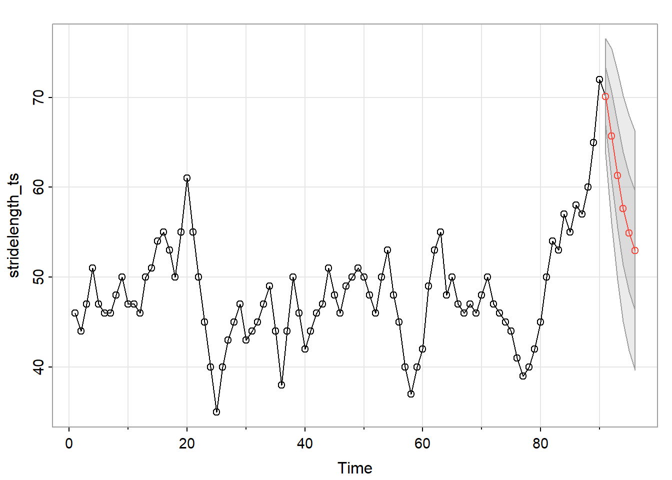
sarima.for(stridelength_ts, 6, 2, 0, 0) will give forecasts and standard errors of prediction errors for the next six times past the end of the series. Here’s the output (slightly edited to fit here):
$pred
Time Series:
Start = 91
End = 96
Frequency = 1
[1] 70.11332 65.70935 61.28431 57.64387 54.90649 52.94874

$se
Time Series:
Start = 91
End = 96
Frequency = 1
[1] 3.202276 4.861848 5.793396 6.280069 6.521255 6.635993
The forecasts are given in the first batch of values under $pred and the standard errors of the forecast errors are given in the last line in the batch of results under $se.
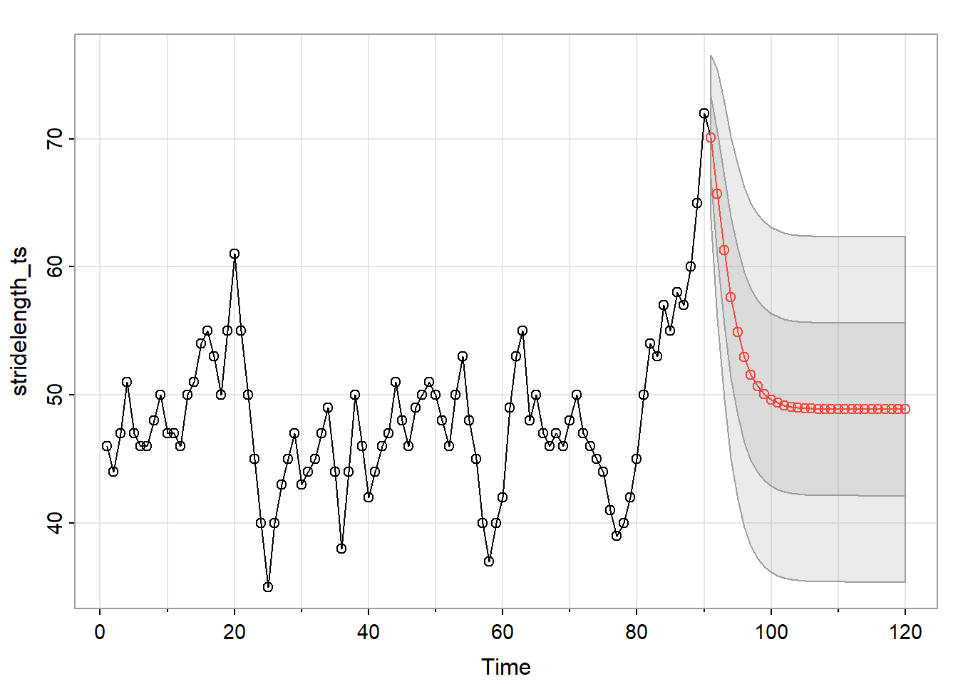
The procedure also gave this graph, which shows the series followed by the forecasts as a red line and the upper and lower prediction limits as blue dashed lines:
Psi-Weights for the Estimated AR(2) for the Stride Length Data
If we wanted to verify the standard error calculations for the six forecasts past the end of the series, we would need to know the psi-weights. To get them, we need to supply the estimated AR coefficients for the AR(2) model to the ARMAtoMA command.
The R command in this case is:
ARMAtoMA(ar = list(1.148, -0.3359), ma = 0, 5)This will give the psi-weights \(\psi_1\) to \(\psi_5\) in scientific notation. The answer provided by R is:
[1] 1.1480000 0.9820040 0.7417274 0.5216479 0.3497056(Remember that \(\psi_0\equiv 1\)in all cases)
The output for estimating the AR(2) included this estimate of the error variance:
sigma^2 estimated as 11.47As an example, the standard error of the forecast error for 3 times past the end of the series is
\[\sqrt{\widehat{\sigma}^2_w\sum_{j=0}^{3-1}\psi^2_j} =\sqrt{11.47(1+1.148^2+0.982^2)} = 6.1357\]
which, except for round off error, matches the value of 6.135493 given as the third standard error in the sarima.for output above.
Where will the Forecasts end up?
For a stationary series and model, the forecasts of future values will eventually converge to the mean and then stay there. Note below what happened with the stride length forecasts, when we asked for 30 forecasts past the end of the series. [Command was sarima.for (stridelength, 30, 2, 0, 0)]. The forecast got to 48.876 and then stayed there.
$pred:Time Series:
Start = 91
End = 120
Frequency = 1
[1] 70.11332 65.70935 61.28431 57.64387 54.90649 52.94874 51.59154 50.66998
[9] 50.05316 49.64455 49.37589 49.20023 49.08586 49.01164 48.96358 48.93252
[17] 48.91248 48.89956 48.89124 48.88589 48.88244 48.88023 48.87880 48.87789
[25] 48.87730 48.87692 48.87668 48.87652 48.87642 48.87636The graph showing the series and the six prediction intervals is the following