13 Fractional Differencing and Threshold Models
ARFIMA
Threshold Models
In this lesson, we’ll look at two variations of ARIMA models - long memory models (fractional differences) and threshold models (regime switching models).
Objectives
Upon completion of this lesson, you should be able to:
- Identify and interpret simple fractionally differenced models
- Recognize when to take first differences vs. fractional differences
- Identify and interpret ARFIMA models
- Apply different models within two intervals of a time series
13.1 Long Memory Models and Fractional Differences
Section 5.1 of Shumway and Stoffer gives a brief overview of “long memory ARMA” models. This type of model may possibly be used when the ACF of the series tapers slowly to 0.
The usual solution in this situation is to explore the first differences of the series. Often, data for which a first difference is successful will typically have a first lag autocorrelation quite close to 1.
In this formulation, we have a first lag AR type of term with a coefficient equal to 1. This creates a first order autocorrelation for the original series close to 1.
In some instances, however, we may see a persistent pattern of non-zero correlations that begins with a first lag correlation that is not close to 1. In these cases, models that incorporate “fractional differencing” may be useful. A simple model that utilizes fractional differencing is
\[(1-B)^dx_t = w_t\]
where d is a value such that \(|d| < .5\) and \(w_t\) is the usual white noise term.
Mathematically, this model can be expanded to be an infinite order AR with coefficients that may taper (very) slowly toward 0. We’ll skip those details (the results are given in our text).
In a fractionally differenced model, the difference coefficient d is a parameter to be estimated. The R package arfima can be used to do this. Again, an indication that this model might be useful is a slowly tapering sample ACF without particularly high autocorrelations.
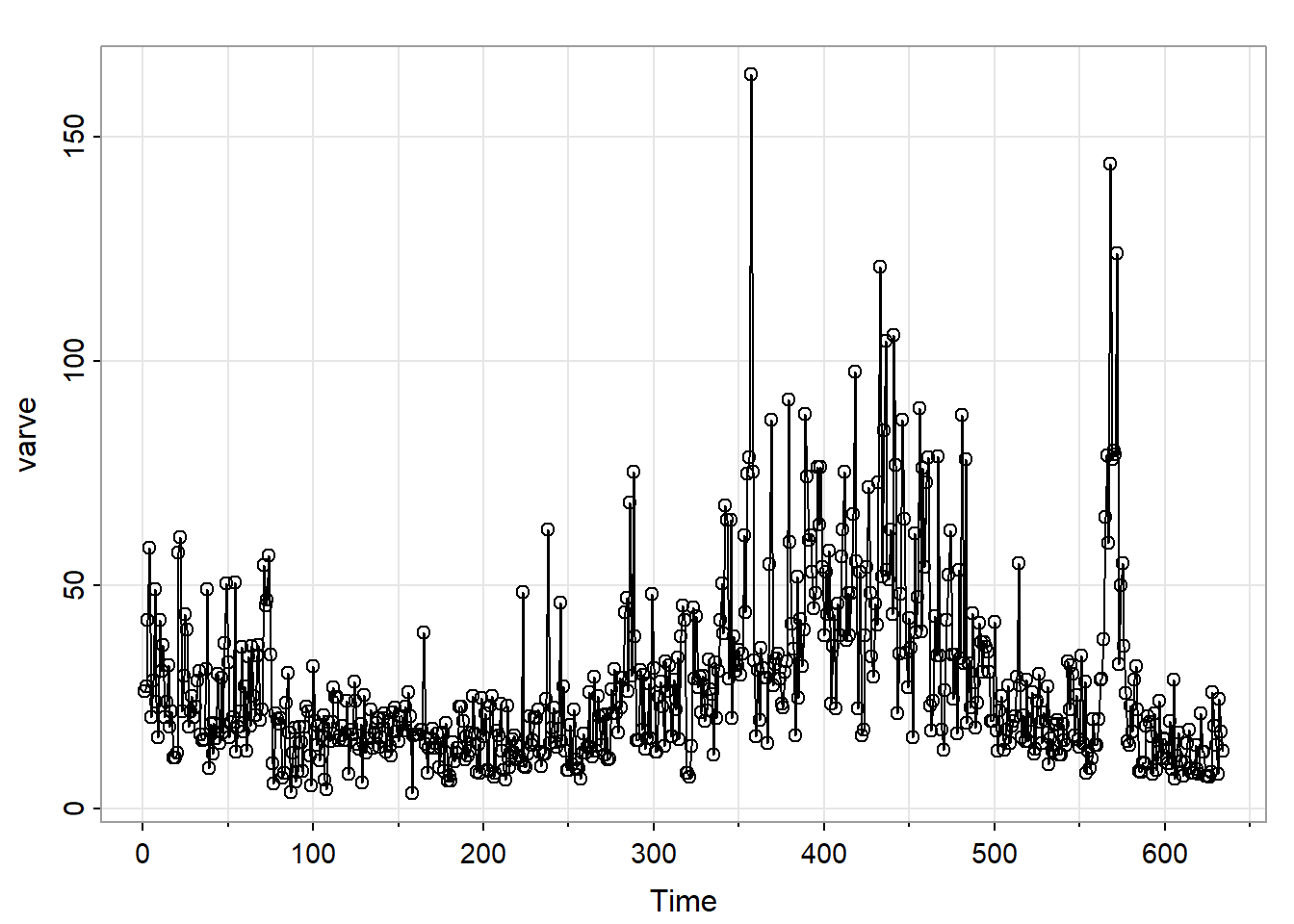
Example 5.1 in the text looks at a fractionally differenced model for a series of n = 634 (yearly) values of a geological measurement called varve. This is a sedimentary layer of sand and silt left by melting glaciers. A time series plot of the data follows.
Due to the period of more extreme variability, the authors suggest analyzing the logarithm of the data. (This might stabilize the variance.)
A plot of the log-transformed series follows:
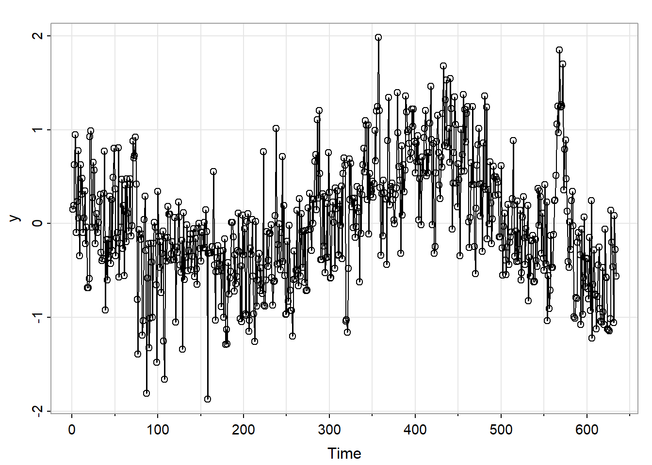
The sample ACF of the log-transformed data shows a persistent pattern of moderately high values. Here’s both the ACF and the PACF. In Chapter 3 of the text the authors use first differencing and explore the relative merits of ARIMA(0,1,1) and ARIMA(1,1,1) models for these data. In Section 5.1, the authors explore a fractionally differenced model.
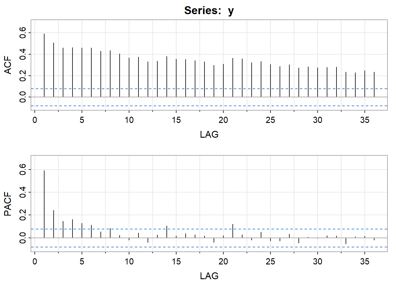
The arfima package gives an estimate for the differencing fraction of \(\widehat{d} = 0.373\). Thus the estimated model is \((1-B)^{.373}x_t = w_t\) where \(x_t\) is the centered log-transformed log series.
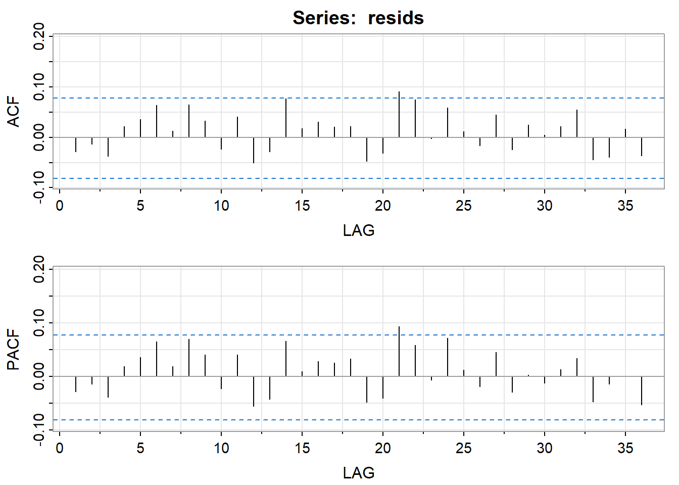
This model provides a good fit to the data as evidenced by the following ACF and PACF of the residuals.
Generalizations
The model can be expanded to include AR and MA terms as well as the fractional difference. These models are called ARFIMA models. To identify an ARFIMA model, we first use the simple fractional difference model \((1-B)^dx_t = w_t\) and then explore the ACF and PACF of the residuals from this model. This is analogous to exploring the ACF and PACF of the first differences when we carry out the usual steps for non-stationary data. The arfima package can be used to fit general ARFIMA models.
Interpretation Difficulty
The main difficulty is that a fractional difference is difficult to interpret. Basically it’s a mathematical device that is used to expand a model into a high-order AR with autocorrelations that match the persistent ”long memory” pattern of the ACF of the series.
R Code
For the following code to run, you have to install the arfima package; this is strongly encouraged over the fracdiff package covered in the text R Code Used in the Example - tsa4. Once the package is installed on your system, you can skip the installation step and use library(arfima) just as we have for the astsa library.
varve = scan("varve.dat")
varve = ts(varve)
library(astsa)
install.packages("arfima")
library(arfima)

y = log(varve) - mean(log(varve)) # Center the logs
acf2(y) ## ACF and PACF of the data

## Estimate d:
varvefd = arfima(y)
summary(varvefd)
d = summary(varvefd)$coef[[1]][1]   #d = 0.3727
d   #prints the value of d to the screen
se.d = summary(varvefd)$coef[[1]][1,2]   #se = 0.0273
se.d   #prints the standard error of d to the screen

##Residuals

resids = resid(varvefd)[[1]]
#resid(varvefd) is a list and [[1]] accesses the residuals as a vector
plot.ts(resids)
acf2(resids)
13.2 Threshold Models
Threshold models are used in several different areas of statistics, not just time series. The general idea is that a process may behave differently when the values of a variable exceed a certain threshold. That is, a different model may apply when values are greater than a threshold than when they are below the threshold. In drug toxicology applications, for example, it may be that all doses below a threshold amount are safe whereas there is increasing toxicity as the dose is increased above the threshold amount. Or, in an animal population abundance study, the population may slowly increase up to a threshold size but then may rapidly decrease (due to limited food) once the population exceeds a certain size.
Threshold models are a special case of regime switching models (RSM). In RSM modeling, different models apply to different intervals of values of some key variable(s).
Section 5.4 of our text discusses threshold autoregressive models (TAR) for univariate time series. In a TAR model, AR models are estimated separately in two or more intervals of values as defined by the dependent variable. These AR models may or may not be of the same order. For convenience, it’s often assumed that they are of the same order.
The text considers only a single threshold value so that there will be two separate AR models – one for values that exceed the threshold and one for values that do not. The difficulties are determining the need for a TAR model, the threshold value to use, and the order(s) of the AR models. One feature for data that a TAR model may work is that the rates of increase and/or decrease may differ when the values are above some level than when the values are below that level.
The estimation of the threshold level is more or less subjective. Many analysts explore several different threshold levels in an attempt to provide a good fit to the data (as measured by MSE values and general features of the residuals). The order(s) of the AR model(s) can also be a trial and error expedition, especially when the inherent model for the data may not be an AR. Generally analysts start with what they think may be a higher order than necessary and then reduce the order as necessary.
Section 5.4 of the text covers threshold models and includes a nice example. In this lesson, we’ll discuss the example and provide the R code. The series for the example is monthly rates of deaths due to flu in the United States for 11 years (n = 132). Due to the epidemic nature of the flu, the behavior of the series is quite different when the rates go above some threshold value than when it’s below the value.
The first step (always) is to plot the data. Following is the time series plot of the data.
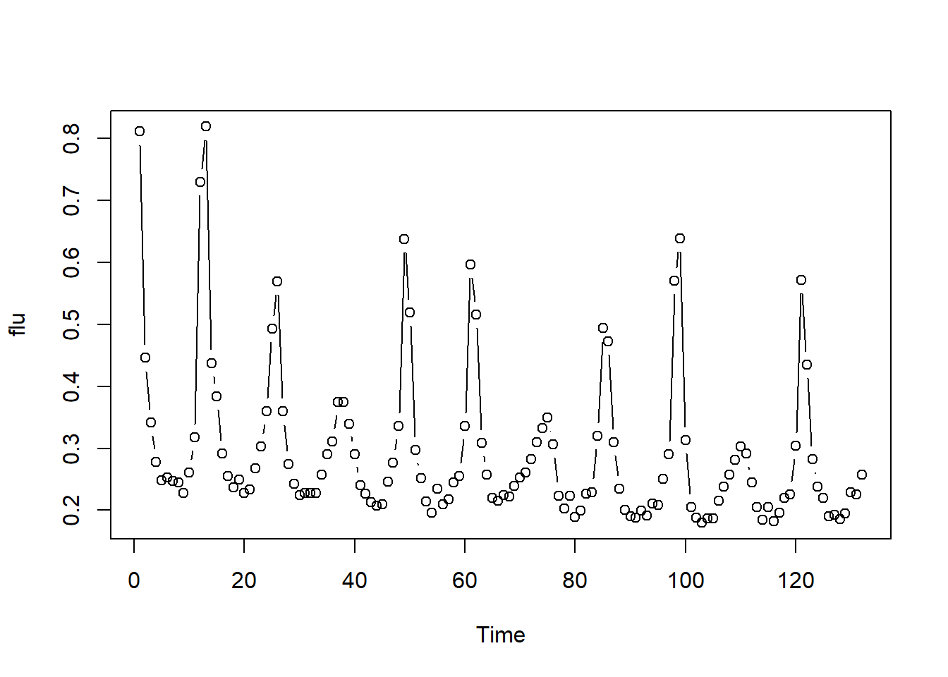
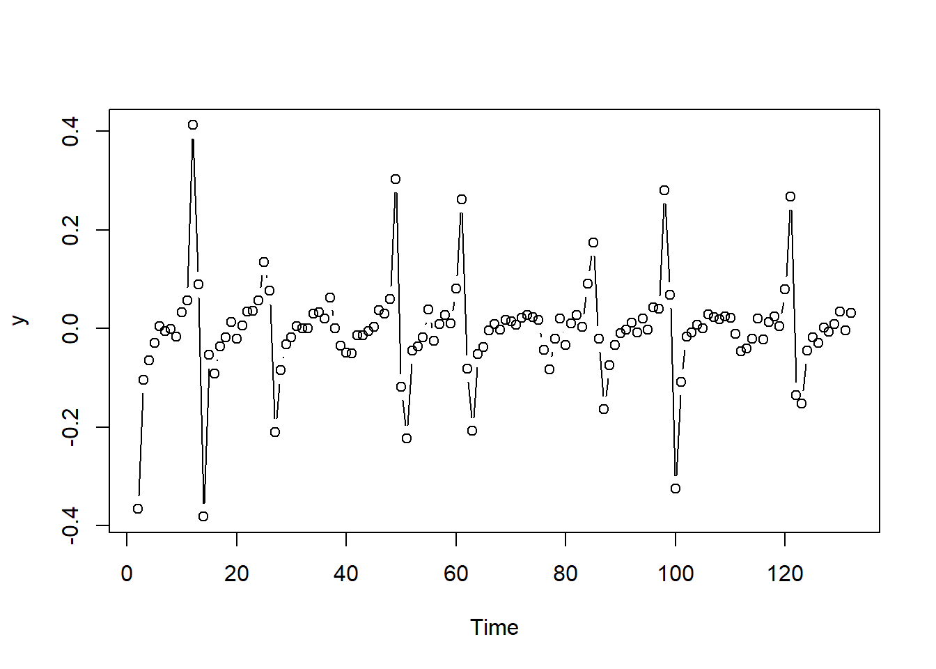
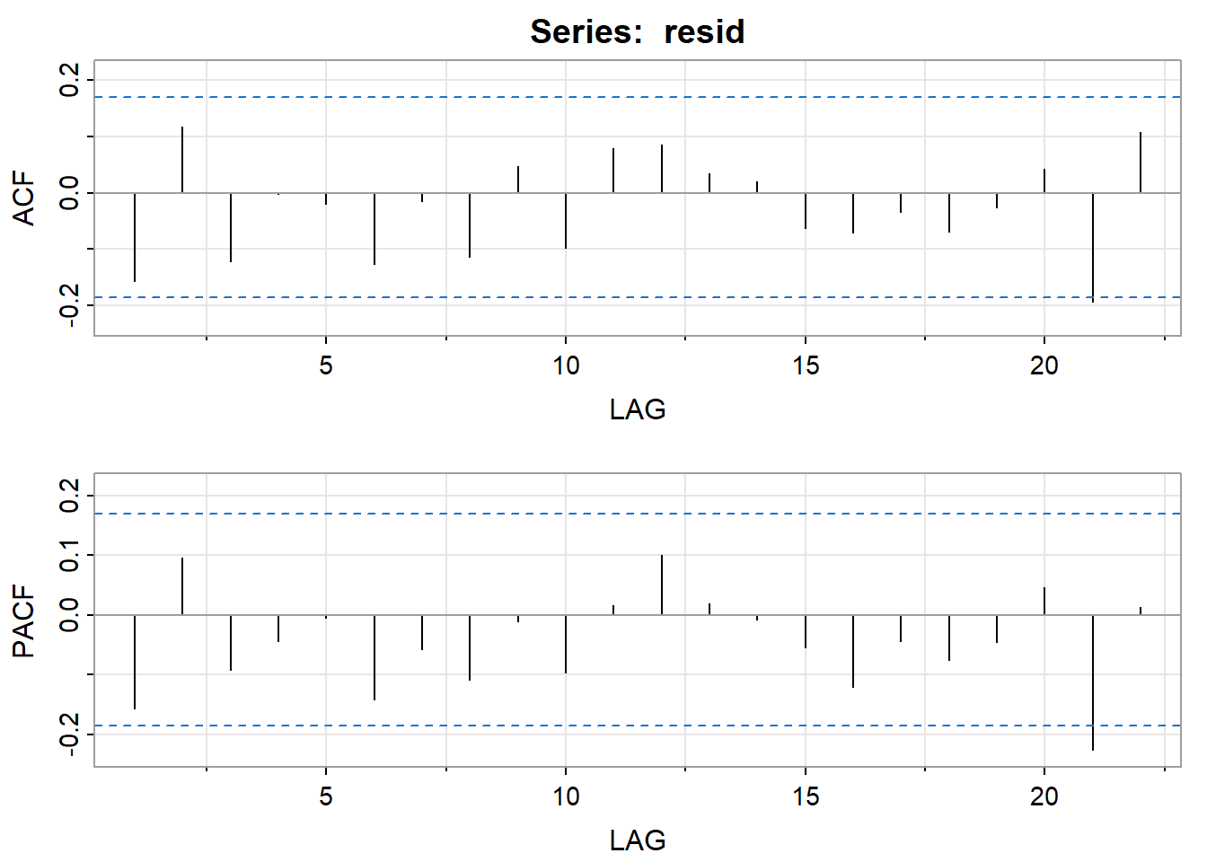
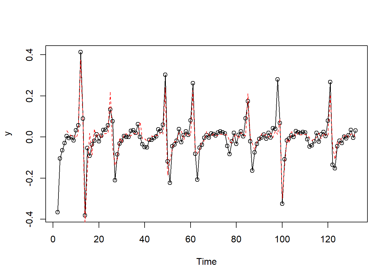
Consistent with the original data, we see sharp increases and decreases in certain periods. After some experimentation the authors decided to use separate AR(4) models for two regions: data following a first difference greater than or equal to .05 and data following a first difference less than .05. The model fit well, as evidence by the following plots – the ACF and PACF of the residuals and a plot comparing actual first difference to predicted first differences. In the plot comparing actual and predicted values, the predicted values are along the red dashed line.
R Code
R code for the example follows. Within the ts.intersect command the lag(,) commands create lags and the matrix that is output will not contain rows with missing values. In the code, we do a regression fit of an AR(4) model for all of the data in order to set up variables that will be used in the separate regime regressions.
library(astsa)
flu = scan("flu.dat")
flu = ts(flu)
plot(flu,type="b")
y = diff(flu,1)
plot(y,type="b")

model = ts.intersect(y, lag1y=lag(y,-1), lag2y=lag(y, -2), lag3y=lag(y,-3), lag4y=lag(y, -4))
x = model[,1]
P = model[,2:5]
c = .05 ## Threshold value

##Regression for values below the threshold
less = (P[,1]<c)
x1 = x[less]
P1 = P[less,]
out1 = lm(x1~P1[,1]+P1[,2]+P1[,3]+P1[,4])
summary(out1)

##Regression for values above the threshold
greater = (P[,1]>=c)
x2 = x[greater]
P2 = P[greater,]
out2 = lm(x2~P2[,1]+P2[,2]+P2[,3]+P2[,4])
summary(out2)

##Residuals
res1 = residuals(out1)
res2 = residuals(out2)
less[less==1]= res1
greater[greater==1] = res2
resid = less + greater
acf2(resid)

##Predicted values
less = (P[,1]<c)
greater = (P[,1]>=c)
fit1 = predict(out1)
fit2 = predict(out2)
less[less==1]= fit1
greater[greater==1] = fit2
fit = less + greater
plot(y, type="o")
lines(fit, col = "red", lty="dashed")
The tsDyn package in R has simplified this code into a handful of steps:
install.packages("tsDyn") #if not yet installed
library(tsDyn)
flu.tar4.05=setar(dflu, m=4, thDelay=0, th=.05) #dflu=diff(flu,1) as given in the text
summary(flu.tar4.05) #this shows the final model above and below .05
plot(flu.tar4.05) #cycles through fit and diagnostic plots
If we do not provide a threshold to the th option, setar searches over a grid to choose a threshold (.036):
flu.tar4=setar(dflu, m=4, thDelay=0)
summary(flu.tar4)
plot(flu.tar4)