11 Vector Autoregressive Models/ ARCH Models
Vector Autoregressive Models
ARCH/GARCH Models
Trend-stationary
Stationary
In this lesson, we’ll look at two topics - models for periods of volatile variance (ARCH models) and AR models for multivariate time series.
Objectives
Upon completion of this lesson, you should be able to:
- Model the variance of a time series
- Identify and interpret ARCH models
- Simultaneously model multiple variables in terms of past lags of themselves and one another
11.1 ARCH/GARCH Models
An ARCH (autoregressive conditionally heteroscedastic) model is a model for the variance of a time series. ARCH models are used to describe a changing, possibly volatile variance. Although an ARCH model could possibly be used to describe a gradually increasing variance over time, most often it is used in situations in which there may be short periods of increased variation. (Gradually increasing variance connected to a gradually increasing mean level might be better handled by transforming the variable.)
ARCH models were created in the context of econometric and finance problems having to do with the amount that investments or stocks increase (or decrease) per time period, so there’s a tendency to describe them as models for that type of variable. For that reason, the authors of our text suggest that the variable of interest in these problems might either be \(y_t=(x_{t}-x_{t-1})/x_{t-1},\) the proportion gained or lost since the last time, or \(log (x_t / x_{t-1})=log(x_t)-log(x_{t-1}),\) the logarithm of the ratio of this time’s value to last time’s value. It’s not necessary that one of these be the primary variable of interest. An ARCH model could be used for any series that has periods of increased or decreased variance. This might, for example, be a property of residuals after an ARIMA model has been fit to the data.
The ARCH(1) Variance Model
Suppose that we are modeling the variance of a series \(y_t\) . The ARCH(1) model for the variance of model \(y_t\) is that conditional on \(y_{t-1}\) , the variance at time \(t\) is
\[\tag{1} \text{Var}(y_t | y_{t-1}) = \sigma^2_t = \alpha_0 + \alpha_1 y^2_{t-1}\]
We impose the constraints \(\alpha_0≥ 0\) and \(\alpha_1 ≥ 0\) to avoid negative variance.
If we assume that the series has mean = 0 (this can always be done by centering), the ARCH model could be written as
\[\tag{2} y_t = \sigma_t \epsilon_t,\]
\[\text{with } \sigma_t = \sqrt{\alpha_0 + \alpha_1y^2_{t-1}},\]
\[\text{and } \epsilon_t \overset{iid}{\sim} (\mu=0,\sigma^2=1)\]
For inference (and maximum likelihood estimation) we would also assume that the \(\epsilon_t\) are normally distributed.
Possibly Useful Results
Two potentially useful properties of the useful theoretical property of the ARCH(1) model as written in equation line (2) above are the following:
\(y^2_t\)has the AR(1) model \(y^2_t = \alpha_0 +\alpha_1y^2_{t-1}+\text{error}.\)
This model will be causal, meaning it can be converted to a legitimate infinite order MA only when \(\alpha^2_1 < \frac{1}{3}\)
\(y_t\)is white noise when 0 ≤ \(\alpha_1\) ≤ 1.
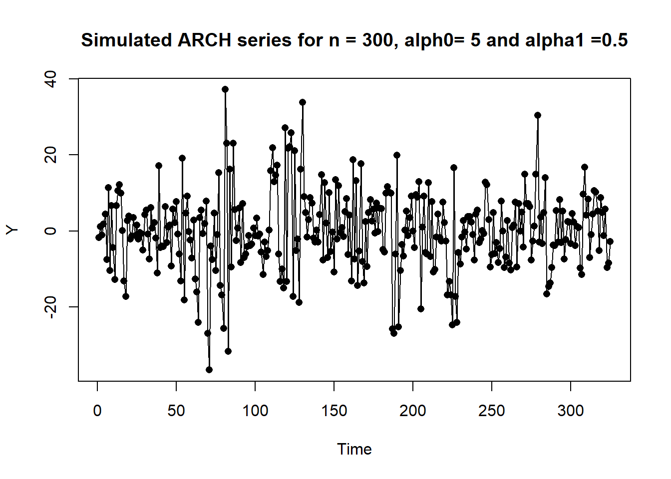
Example 11.1 The following plot is a time series plot of a simulated series (n = 300) for the ARCH model
\[\text{Var}(y_t | y_{t-1}) = \sigma^2_t = 5 + 0.5y^2_{t-1}.\]
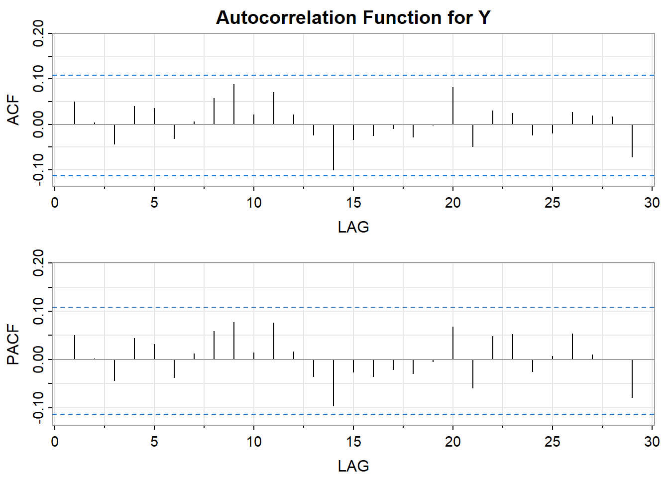
The ACF of this series just plotted follows:
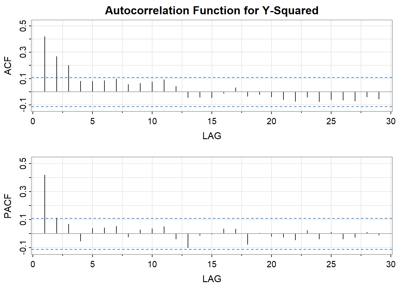
The PACF (above) of the squared values has a single spike at lag 1 while the ACF tapers suggesting an AR(1) model for the squared series.
Generalizations
An ARCH(m) process is one for which the variance at time \(t\) is conditional on observations at the previous m times, and the relationship is
\[\text{Var}(y_t | y_{t-1}, \dots, y_{t-m}) = \sigma^2_t = \alpha_0 + \alpha_1y^2_{t-1} + \dots + \alpha_my^2_{t-m}.\]
With certain constraints imposed on the coefficients, the \(y_t\) series squared will theoretically be AR(m).
A GARCH (generalized autoregressive conditionally heteroscedastic) model uses values of the past squared observations and past variances to model the variance at time \(t.\) As an example, a GARCH(1,1) is
\[\sigma^2_t = \alpha_0 + \alpha_1 y^2_{t-1} + \beta_1\sigma^2_{t-1}\]
In the GARCH notation, the first subscript refers to the order of the \(y^2\) terms on the right side, and the second subscript refers to the order of the \(\sigma^2\) terms.
Identifying an ARCH/GARCH Model in Practice
The best identification tool may be a time series plot of the series. It’s usually easy to spot periods of increased variation sprinkled through the series. It can be fruitful to look at the ACF and PACF of both \(y_t\) and \(y^2_t.\) For instance, if \(y_t\) appears to be white noise and \(y^2_t\) appears to be AR(1), then an ARCH(1) model for the variance is suggested. If the PACF of the \(y^2_t\) suggests AR(m), then ARCH(m) may work. GARCH models may be suggested by an ARMA type look to the ACF and PACF of \(y^2_t.\) In practice, things won’t always fall into place as nicely as they did for the simulated example in this lesson. You might have to experiment with various ARCH and GARCH structures after spotting the need in the time series plot of the series.
In the book, read Example 5.4 (an AR(1)-ARCH(1)), and Example 5.5 (GARCH(1,1)). R code for will also be given in the homework for this week.
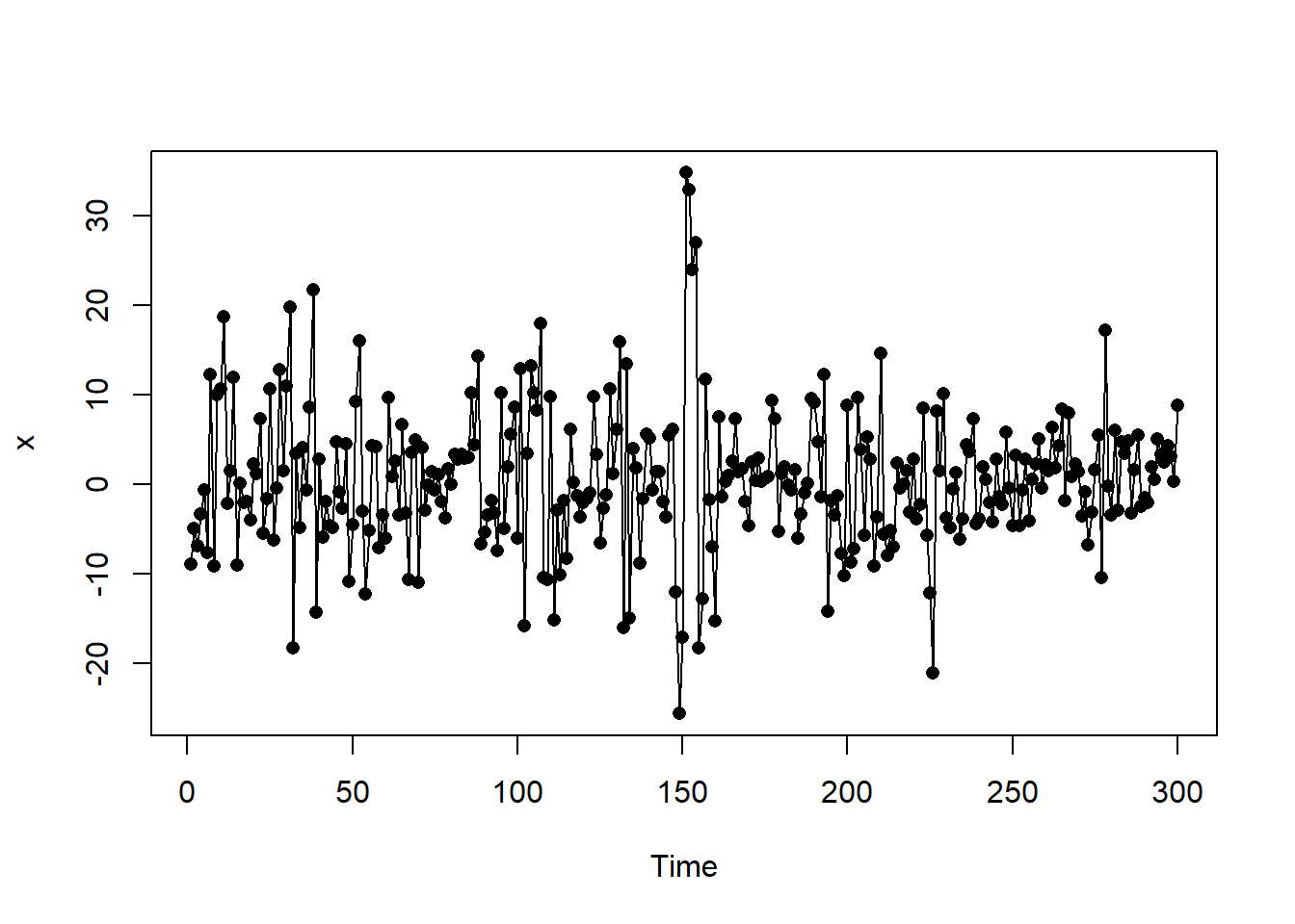
Example 11.2 The following plot is a time series plot of a simulated series, \(x,\) (n = 300) for the GARCH(1,1) model
\[\text{Var}(x_t | x_{t-1}) = \sigma^2_t = 5 + 0.5x^2_{t-1} + 0.5 \sigma^2_{t-1}\]
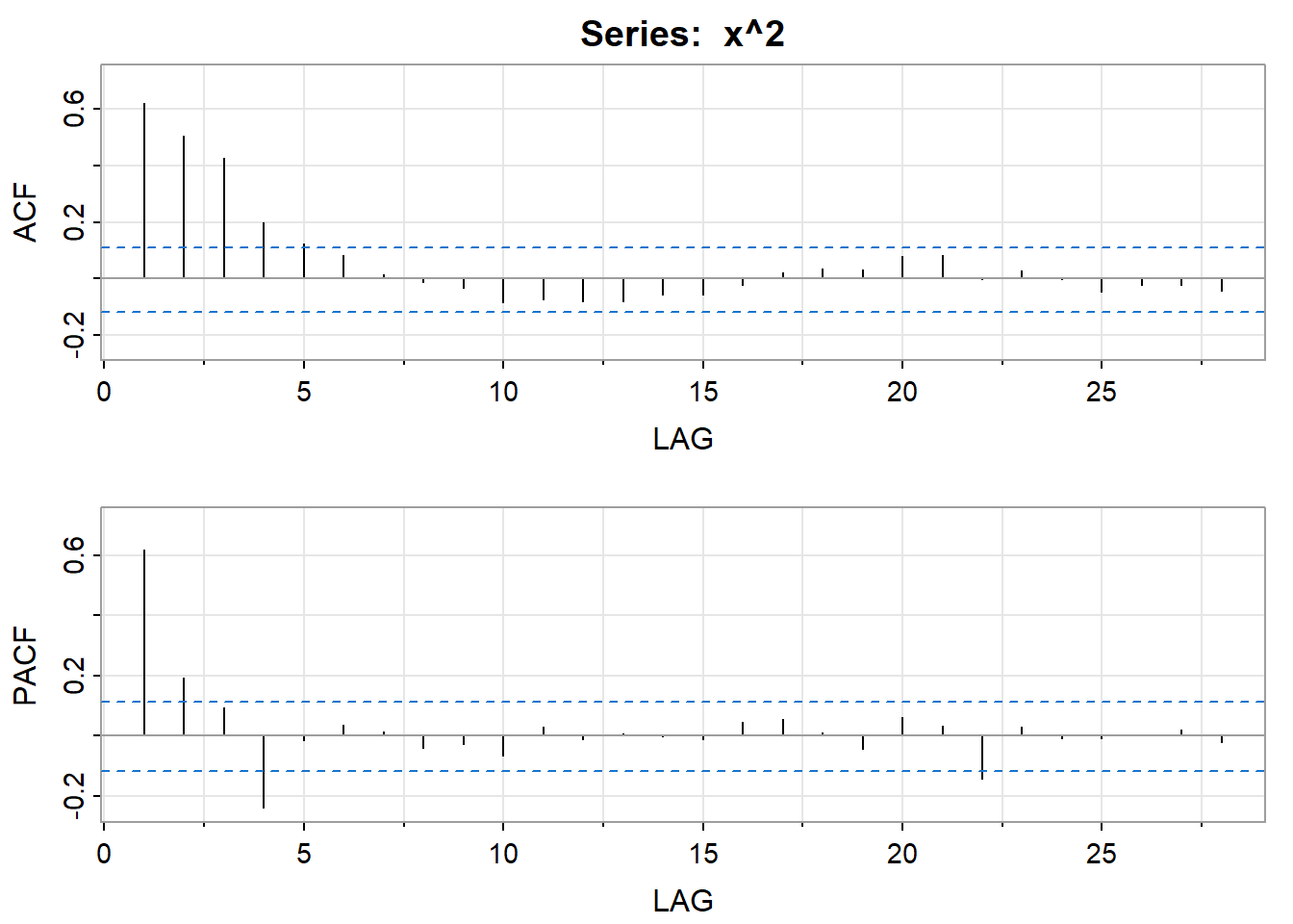
The ACF of the series below shows that the series looks to be white noise.
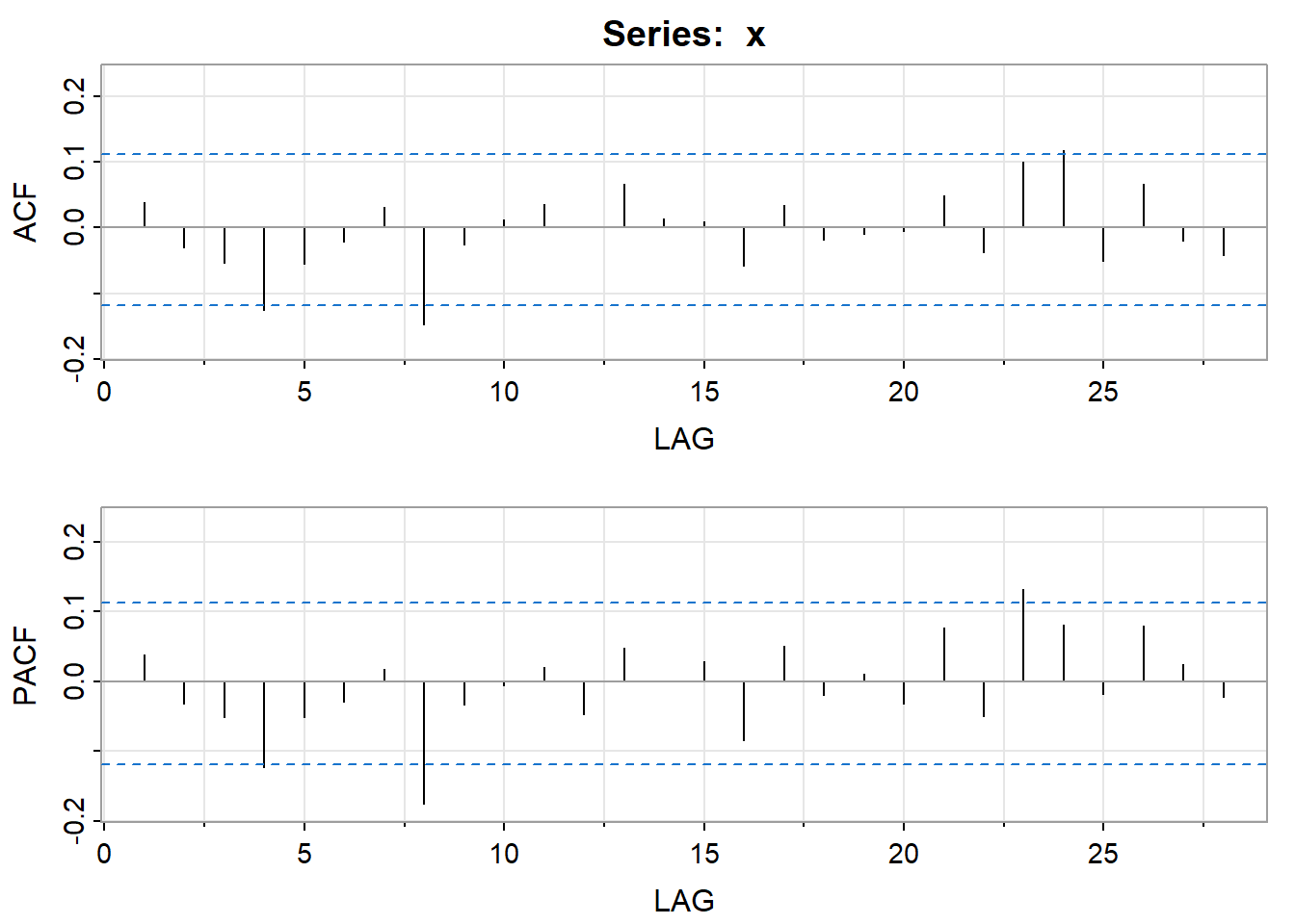
The ACF of the squared series follows an ARMA pattern because both the ACF and PACF taper. This suggests a GARCH(1,1) model.
Let’s use the fGarch package to fit a GARCH(1,1) model to x where we center the series to work with a mean of 0 as discussed above.
install.packages("fGarch") #If not already installed
library(fGarch)
y = x - mean(x) #center x ; mean(x) = 0.5423
x.g = garchFit(~garch(1,1), y, include.mean=F)
summary(x.g)
Here is part of the output:
         Estimate  Std. Error  t value     Pr(>|t|)
omega  10.1994158   3.2571518 3.131391 1.739804e-03
alpha1  0.5093218   0.1114673 4.569250 4.894734e-06
beta1   0.3526627   0.1040485 3.389405 7.004446e-04
This suggests the following model for \(y_t = x_t - 0.5423\):
The fGarch summary provides the Jarque Bera Test for the null hypothesis that the residuals are normally distributed and the familiar Ljung-Box Tests. Ideally all p-values are above 0.05.
Here are the Standardized Residuals Tests:
Standardised Residuals Tests:
                                 Statistic    p-Value
 Jarque-Bera Test   R    Chi^2   3.4856989 0.17502097
 Shapiro-Wilk Test  R    W       0.9908482 0.05851528
 Ljung-Box Test     R    Q(10)   8.1195466 0.61716095
 Ljung-Box Test     R    Q(15)  10.6948542 0.77391049
 Ljung-Box Test     R    Q(20)  11.6488559 0.92763205
 Ljung-Box Test     R^2  Q(10)   7.4634615 0.68108565
 Ljung-Box Test     R^2  Q(15)   8.8929303 0.88304888
 Ljung-Box Test     R^2  Q(20)  14.9066712 0.78172276
 LM Arch Test       R    TR^2    7.1462344 0.84780031

Information Criterion Statistics:
     AIC      BIC      SIC     HQIC
6.641594 6.678631 6.641396 6.656416
Diagnostics all look okay.
11.2 Vector Autoregressive models VAR(p) models
VAR models (vector autoregressive models) are used for multivariate time series. The structure is that each variable is a linear function of past lags of itself and past lags of the other variables.
As an example suppose that we measure three different time series variables, denoted by \(x_{t,1},\) \(x_{t,2},\) and \(x_{t,3}.\)
The vector autoregressive model of order 1, denoted as VAR(1), is as follows:
\[x_{t,1} = \alpha_{1} + \phi_{11} x_{t−1,1} + \phi_{12}x_{t−1,2} + \phi_{13}x_{t−1,3} + w_{t,1}\]
\[x_{t,2} = \alpha_{2} + \phi_{21} x_{t−1,1} + \phi_{22}x_{t−1,2} + \phi_{23}x_{t−1,3} + w_{t,2}\]
\[x_{t,3} = \alpha_{3} + \phi_{31} x_{t−1,1} + \phi_{32}x_{t−1,2} + \phi_{33}x_{t−1,3} + w_{t,3}\]
Each variable is a linear function of the lag 1 values for all variables in the set.
In a VAR(2) model, the lag 2 values for all variables are added to the right sides of the equations, In the case of three x-variables (or time series) there would be six predictors on the right side of each equation, three lag 1 terms and three lag 2 terms.
In general, for a VAR(p) model, the first p lags of each variable in the system would be used as regression predictors for each variable.
VAR models are a specific case of more general VARMA models. VARMA models for multivariate time series include the VAR structure above along with moving average terms for each variable. More generally yet, these are special cases of ARMAX models that allow for the addition of other predictors that are outside the multivariate set of principal interest.
Here, as in Section 5.6 of the text, we’ll focus on VAR models.
On page 304, the authors fit the model of the form
\[\mathbf{x}_t = \Gamma \mathbf{u}_t + \phi \mathbf{x}_{t-1} + \mathbf{w}_t\]
where \(\mathbf{u}_t = (1, t)’\) includes terms to simultaneously fit the constant and trend. It arose from macroeconomic data where large changes in the data permanently affect the level of the series.
There is a not so subtle difference here from previous lessons in that we now are fitting a model to data that need not be stationary. In previous versions of the text, the authors separately de-trended each series using a linear regression with \(t,\) the index of time, as the predictor variable. The de-trended values for each of the three series are the residuals from this linear regression on \(t.\) The de-trending is useful conceptually because it takes away the common steering force that time may have on each series and created stationarity as we have seen in past lessons. This approach results in similar coefficients, though slightly different as we are now simultaneously fitting the intercept and trend together in a multivariate OLS model.
The R vars library authored by Bernhard Pfaff has the capability to fit this model with trend. Let’s look at 2 examples: a trend-stationary model and a stationary model.
Trend-Stationary Model
Example 5.10 from the text is a trend-stationary model in that the de-trended series are stationary. We need not de-trend each series as described above because we can include the trend directly in the VAR model with the VAR command. Let’s examine the code and example from the text by fitting the model above:
install.packages("vars") #If not already installed
install.packages("astsa") #If not already installed
library(vars)
library(astsa)
x = cbind(cmort, tempr, part)
plot.ts(x , main = "", xlab = "")
fitvar1= VAR(x, p=1, type="both")
summary(fitvar1)- The first two commands load the necessary commands from the vars library and the necessary data from our text’s library.
- The
cbindcommand creates a vector of response variables (a necessary step for multivariate responses). - The
VARcommand does estimation of AR models using ordinary least squares while simultaneously fitting the trend, intercept, and ARIMA model. Thep = 1argument requests an AR(1) structure and “both” fits constant and trend. With the vector of responses, it’s actually aVAR(1).
Following is the output from the VAR command for the variable tempr (the text provides the output for cmort):
             Estimate  Std. Error   t value     Pr(>|t|)
cmort.l1 -0.244046444 0.042104647 -5.796188 1.199814e-08
tempr.l1  0.486595619 0.036899471 13.187062 2.630720e-34
part.l1  -0.127660994 0.021985184 -5.806683 1.131454e-08
const    67.585597743 5.541549825 12.196154 3.795836e-30
trend    -0.006912455 0.002267963 -3.047869 2.426171e-03
The coefficients for a variable are listed in the Estimate column. The .l1 attached to each variable name indicates that they are lag 1 variables.
Using notation T = temperature, t=time (collected weekly), M = mortality rate, and P = pollution, the equation for temperature is
\[\widehat{T}_t = 67.586 - .007 t - 0.244 M_{t-1} + 0.487 T_{t-1} - 0.128 P_{t-1}\]
The equation for mortality rate is
\[\widehat{M}_t = 73.227 – 0.014 t + 0.465 M_{t-1} - 0.361 T_{t-1} + 0.099 P_{t-1}\]
The equation for pollution is
\[\widehat{P}_t = 67.464 - .005 t - 0.125 M_{t-1} - 0.477 T_{t-1} +0.581 P_{t-1}.\]
The covariance matrix of the residuals from the VAR(1) for the three variables is printed below the estimation results. The variances are down the diagonal and could possibly be used to compare this model to higher order VARs. The determinant of that matrix is used in the calculation of the BIC statistic that can be used to compare the fit of the model to the fit of other models (see formulas 5.89 and 5.90 of the text).
For further references on this technique see Analysis of integrated and co-integrated time series with R by Pfaff and also Campbell and Perron [1991].
In Example 5.11, the authors give results for a VAR(2) model for the mortality rate data. In R, you may fit the VAR(2) model with the command summary(VAR(x, p=2, type="both")).
summary(VAR(x, p=2, type="both"))$varresult$temprThe output, as displayed by the VAR command is as follows:
Call:
lm(formula = y ~ -1 + ., data = datamat)

Residuals:
    Min      1Q  Median      3Q     Max
-19.108  -4.093  -0.266   3.669  21.667

Coefficients:
          Estimate Std. Error t value Pr(>|t|)
cmort.l1 -0.108889   0.050667  -2.149  0.03211 *
tempr.l1  0.260963   0.051292   5.088 5.14e-07 ***
part.l1  -0.050542   0.027844  -1.815  0.07010 .
cmort.l2 -0.040870   0.048587  -0.841  0.40065
tempr.l2  0.355592   0.051762   6.870 1.93e-11 ***
part.l2  -0.095114   0.029295  -3.247  0.00125 **
const    49.880485   6.854540   7.277 1.34e-12 ***
trend    -0.004754   0.002308  -2.060  0.03993 *
---
Signif. codes:  0 '***' 0.001 '**' 0.01 '*' 0.05 '.' 0.1 ' ' 1

Residual standard error: 6.134 on 498 degrees of freedom
Multiple R-squared:  0.5445,    Adjusted R-squared:  0.5381
F-statistic: 85.04 on 7 and 498 DF,  p-value: < 2.2e-16
Again, the coefficients for a particular variable are listed in the Estimate column. As an example, the estimated equation for temperature is
\[\widehat{T}_t = 49.88 - .005 t - 0.109 M_{t-1} + 0.261 T_{t-1} – 0.051 P_{t-1} - 0.041 M_{t-2} + 0.356 T_{t-2} – 0.095 P_{t-2}\]
We will discuss information criterion statistics to compare VAR models of different orders in the homework.
Residuals are also available for analysis. For example, if we assign the VAR command to an object titled fitvar2 in our program,
fitvar2 = VAR(x, p=2, type="both")then we have access to the matrix residuals(fitvar2). This matrix will have three columns, one column of residuals for each variable.
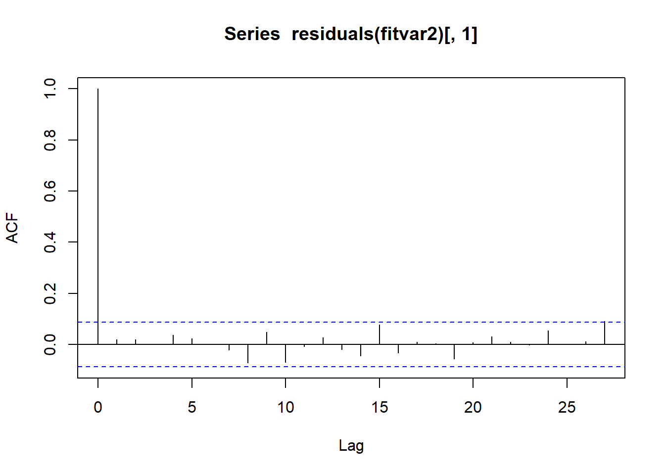
For example, we might use
acf(residuals(fitvar2)[,1])to see the ACF of the residuals for mortality rate after fitting the VAR(2) model.
Following is the ACF that resulted from the command just described. It looks good for a residual ACF. (The big spike at the beginning is the unimportant lag 0 correlation.)
The following two commands will create ACFs for the residuals for the other two variables.
acf(residuals(fitvar2)[,2])
acf(residuals(fitvar2)[,3])
They also resemble white noise.
We may also examine these plots in the cross-correlation matrix provided by acf(residuals(fitvar2)):
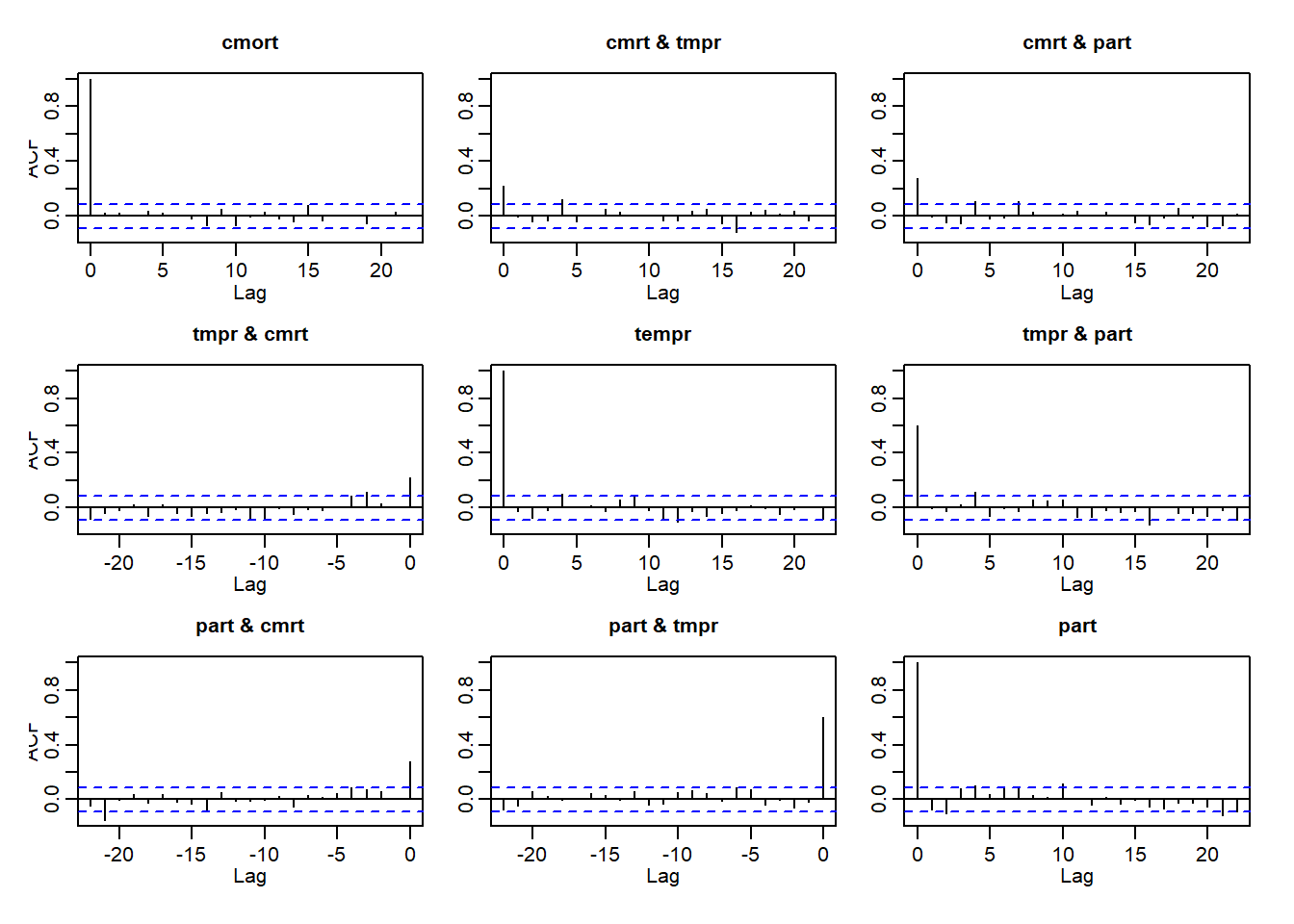
The plots along the diagonal are the individual ACFs for each model’s residuals that we just discussed above. In addition, we now see the cross-correlation plots of each set of residuals. Ideally, these would also resemble white noise at every lag, including lag 0, however we do see remaining cross-correlations, especially between temperature and pollution. As our authors note, this model does not adequately capture the complete association between these variables in time.
Stationary Model
Lets explore an example where the original data are stationary and examine the VAR code by fitting the model above with both a constant and trend. Using R, we simulated n = 500 sample values using the VAR(2) model
\[y_{t,1} = 10 +.25y_{t−1,1} - .20y_{t−1,2} -.40y_{t−2,1} -.65y_{t−2,2}\]
\[y_{t,2} = 20 +.60y_{t−1,1} - .45y_{t−1,2} +.50y_{t−2,1} +.35y_{t−2,2}\]
Using the VAR command explained above:
y1=scan("var2daty1.dat")
y2=scan("var2daty2.dat")
summary(VAR(cbind(y1,y2), p=2, type="both"))
We obtain the following output:
Call:
lm(formula = y ~ -1 + ., data = datamat)

Residuals:
     Min       1Q   Median       3Q      Max
-2.88788 -0.72109  0.01674  0.66900  3.01475

Coefficients:
        Estimate Std. Error t value Pr(>|t|)
y1.l1  0.2936164  0.0296083   9.917  < 2e-16 ***
y2.l1 -0.1899661  0.0372244  -5.103 4.78e-07 ***
y1.l2 -0.4534486  0.0374431 -12.110  < 2e-16 ***
y2.l2 -0.6357889  0.0243282 -26.134  < 2e-16 ***
const  9.5042389  0.8742212  10.872  < 2e-16 ***
trend  0.0001730  0.0003116   0.555    0.579
---
Signif. codes:  0 '***' 0.001 '**' 0.01 '*' 0.05 '.' 0.1 ' ' 1

Residual standard error: 0.9969 on 492 degrees of freedom
Multiple R-squared:  0.8582,    Adjusted R-squared:  0.8568
F-statistic: 595.5 on 5 and 492 DF,  p-value: < 2.2e-16
The estimates are very close to the simulated coefficients and the trend is not significant, as expected. For stationary data, when detrending is unnecessary, you may also use the ar.ols command to fit a VAR model:
fitvar2 = ar.ols(cbind(y1, y2), order=2)
Call:
ar.ols(x = cbind(y1, y2), order.max = 2)

$ar
, , 1

       y1      y2
y1 0.2930 -0.1913
y2 0.6506 -0.3998

, , 2

        y1      y2
y1 -0.4523 -0.6365
y2  0.4534  0.3847


$x.intercept
       y1        y2
-0.043637 -0.003306

$var.pred
        y1      y2
y1 0.98244 0.03339
y2 0.03339 0.96656
In the first matrix given, read across a row to get the coefficients for a variable. The preceding commas followed by 1 or 2 indicate whether the coefficients are lag 1 or lag 2 variables respectively. The intercepts of the equations are given under $x.intercept – one intercept per variable.
The matrix under $var.pred gives the variance-covariance matrix of the residuals from the VAR(2) for the two variables. The variances are down the diagonal and could possibly be used to compare this model to higher order VARs as noted above.
The standard errors of the AR coefficients are given by the fitvar2$asy.se.coef command. The output is:
$x.mean
        y1         y2
0.04443272 0.04407215

$ar
, , y1

          y1         y2
1 0.02941649 0.02917778
2 0.03716747 0.03686586

, , y2

          y1         y2
1 0.03693359 0.03663388
2 0.02415371 0.02395770
As with the coefficients, read across rows. The first row gives the standard errors of the coefficients for the lag 1 variables that predict y1. The second row gives the standard errors for the coefficients that predict y2.
You may note that the coefficients are close to the VAR command except the intercept. This is because ar.ols estimates the model for x-mean(x). To match the intercept provided by the summary(VAR(cbind(y1,y2), p=2, type="const")) command, you must calculate the intercept as follows:
In our example, the intercept for the simulated model for \(y_{t,1}\) equals
and the estimated equation for \(y_{t,1}\)
\[y_{t,1}= 9.58 +.29y_{t−1,1} - .19y_{t−1,2} -.45y_{t−2,1} -.64y_{t−2,2}\]