8 Regression with ARIMA errors, Cross correlation functions, and Relationships between 2 Time Series
Regression with ARIMA errors
CCF
Lagged Regression
Overview
In this lesson, we’ll start coverage of regression between two time series.
Objectives
Upon completion of this lesson, you should be able to:
- Recognize when and how to adjust for residuals with a time series structure
- Estimate the adjusted intercept and slope
- Interpret the cross-correlation function
- Identify and interpret transfer function models
8.1 Linear Regression Models with Autoregressive Errors
When we do regressions using time series variables, it is common for the errors (residuals) to have a time series structure. This violates the usual assumption of independent errors made in ordinary least squares regression. The consequence is that the estimates of coefficients and their standard errors will be wrong if the time series structure of the errors is ignored.
It is possible, though, to adjust estimated regression coefficients and standard errors when the errors have an AR structure. More generally, we will be able to make adjustments when the errors have a general ARIMA structure.
The Regression Model with AR Errors
Suppose that \(y_t\) and \(x_t\) are time series variables. A simple linear regression model with autoregressive errors can be written as
\[y_{t} =\beta_{0}+\beta_{1}x_{t}+\epsilon_{t}\]
with \(\epsilon_t = \phi_{1}\epsilon_{t-1}+\phi_{2}\epsilon_{t-2}+ \cdots + w_t,\) and \(w_t \sim \text{iid}\; N(0, \sigma^2).\)
If we let \(\Phi(B)=1-\phi_{1}B- \phi_{2}B^2 - \cdots,\) then we can write the AR model for the errors as
\[\Phi(B)\epsilon_{t}=w_{t}.\]
If we assume that an inverse operator, \(\Phi^{-1}(B),\) exists, then \(\epsilon_{t}=\Phi^{-1}(B)w_{t}.\)
So, the model can be written
\[y_t =\beta_{0} +\beta_{1}x_{t} + \Phi^{-1}(B)w_{t},\]
where \(w_{t}\) is the usual white noise series.
Examining Whether This Model May Be Necessary
- Start by doing an ordinary regression. Store the residuals.
- Analyze the time series structure of the residuals to determine if they have an AR sructure.
- If the residuals from the ordinary regression appear to have an AR structure, estimate this model and diagnose whether the model is appropriate.
Theory for the Cochrane-Orcutt Procedure
A simple regression model with AR errors can be written as
\[(1) \;\;\; y_t =\beta_0 +\beta_1x_t + \Phi^{-1}(B)w_{t}\]
\(\Phi(B)\) gives the AR polynomial for the errors.
If we multiply all elements of the equation by \(\Phi(B),\) we get
\[\Phi(B)y_t = \Phi(B)\beta_0 +\beta_1\Phi(B)x_t + w_t\]
- Let \(y^{*}_{t} =\Phi(B)y_{t} = y_{t} - \phi_{1}y_{t-1} - \cdots - \phi_{p}y_{t-p}\)
- Let \(x^{*}_{t} =\Phi(B)x_{t} = x_{t} - \phi_{1}x_{t-1} - \cdots - \phi_{p}x_{t-p}\)
- Let \(\beta^{*}_{0} =\Phi(B)\beta_{0} = (1 - \phi_{1} - \cdots - \phi_{p})\beta_{0}\)
Using the items just defined, we can write the model as
\[(2) \;\;\; y^*_t =\beta^*_0 +\beta_1x^*_t + w_{t}\]
Remember that \(w_t\) is a white noise series, so this is just the usual simple regression model.
We use results from model (2) to iteratively adjust our estimates of coefficients in model (1).
- The estimated slope \(\widehat{\beta}_1\) from model (2) will be the adjusted estimate of the slope in model (1) (and its standard error from this model will be correct as well).
- To adjust our estimate of the intercept \(\beta_0\) in model (1), we use the relationship \(\beta^*_0=(1 - \phi_{1} - \cdots - \phi_{p})\beta_{0}\) to determine that \(\widehat{\beta}_0=\dfrac{\widehat{\beta}^*_0}{1 - \widehat{\phi}_{1} - \cdots - \widehat{\phi}_{p}}.\)
The standard error for \(\widehat{\beta}_0\) is \[s.e.( \widehat{\beta}_0) =\dfrac {s.e. ( \widehat{\beta}^{*}_{0})} {1 - \widehat{\phi}_{1} - \cdots - \widehat{\phi}_{p}}.\]
This procedure is attributed to Cochrane and Orcutt (1949) and is repeated until the estimates converge, that is we observe a very small difference in our estimates between iterations.
Additional Comment
For a higher order AR, the adjustment variables are calculated in the same manner with more lags. For instance, suppose the residuals were found to have an AR(2) with estimated coefficients 0.9 and -0.2. Then the y- and x- variables for the adjustment regression would be
\[y^{*}_{t} = y_{t} - 0.9y_{t-1}+0.2y_{t-2}\]
\[x^{*}_{t} = x_{t} - 0.9x_{t-1}+0.2x_{t-2}\]
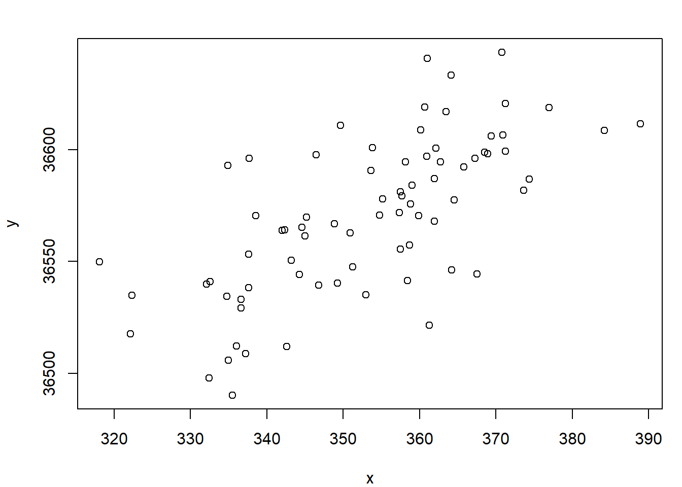
Example 8.1 (Economic Measure) There are n = 76 annual observations in sequence. Suppose x is a leading economic indicator (predictor) for a country and y is a measure of the state of the economy. The following plot shows the relationship between x and y for 76 years.
Suppose that we want to estimate the linear regression relationship between y and x at concurrent times.
Step 1
Estimate the usual regression model. Results from R are:
                Estimate Std. Error    t value      Pr(>|t|)
(Intercept) 36001.842384 71.5206100 503.377172 1.522931e-132
x               1.609842  0.2023281   7.956593  1.564697e-11
(It is not shown, but worth noting that trend=time(x) is not significant in this regression and x is not changing over time.)
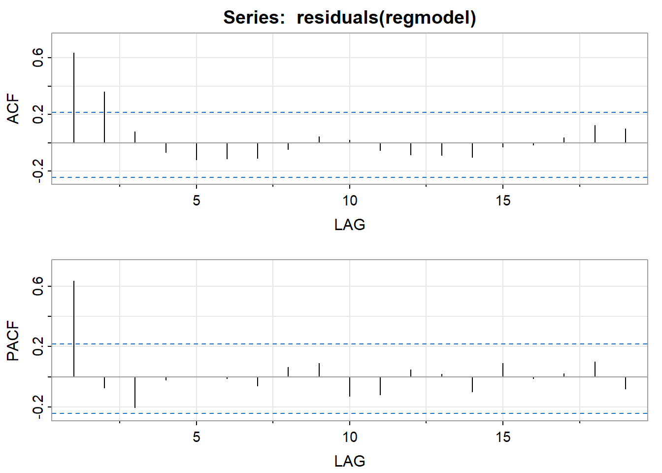
Step 2
Examine the AR structure of the residuals. Following are the ACF and PACF of the residuals. It looks like the errors from Step 1 have an AR(1) structure.
Step 3
Estimate the AR coefficients (and make sure that the AR model actually fits the residuals). For this example, the R estimate of the AR(1) coefficient is 0.6488.
<><><><><><><><><><><><><><>

Coefficients:
    Estimate     SE t.value p.value
ar1   0.6488 0.0875  7.4136       0

sigma^2 estimated as 378.0578 on 75 degrees of freedom

AIC = 8.832745  AICc = 8.833456  BIC = 8.89408
Model diagnostics (not shown here) were okay.
Step 4
Calculate variables to use in the adjustment regression:
\[x^{*}_{t} = x_{t} - 0.6488x_{t-1}\]
\[y^{*}_{t} = y_{t} - 0.6488y_{t-1}\]
Step 5
Use ordinary regression to estimate the model \(y^*_t = \beta^*_0 + \beta_1 x^*_t +w_t.\) For this example, the results are
                Estimate Std. Error   t value      Pr(>|t|)
(Intercept) 12641.293556 14.7592834 856.49779 7.753604e-148
xnew            1.635378  0.1174221  13.92735  3.029353e-22
The slope estimate (1.64) and its standard error (0.1174) are the adjusted estimates for the original model.
The adjusted estimate of the intercept of the original model is \(12640/(1-0.6488) = 35990.\) The estimated standard error of the intercept is \(14.76/(1-0.6488) = 42.03.\)
Iterating this procedure until the estimates converge results in an adjusted slope estimate of 1.635 with a standard error of 0.11805 for the original model.
Thus our estimated relationship between \(y_t\) and \(x_t\) is
\[y_t = 35995 + 1.635x_t\]
The errors have the estimated relationship \(e_t = 0.6384 e_{t-1} + w_t.\)
The R Program
Download the data used in the following code: (econpredictor.dat), (econmeasure.dat)
x=ts(scan("econpredictor.dat"))
y=ts(scan("econmeasure.dat"))
plot.ts(x,y,xy.lines=F,xy.labels=F)

regmodel=lm(y~x)
summary(regmodel)
acf2(residuals(regmodel))

ar1res = sarima (residuals(regmodel), 1,0,0, no.constant=T) #AR(1)
xl = ts.intersect(x, lag(x,-1)) # Create matrix with x and lag 1 x as elements
xnew=xl[,1] - 0.6488*xl[,2] # Create x variable for adjustment regression
yl = ts.intersect(y,lag(y,-1)) # Create matrix with y and lag 1 y as elements
ynew=yl[,1]-0.6488*yl[,2] # Create y variable for adjustment regression

adjustreg = lm(ynew~xnew) # Adjustment regression
summary(adjustreg)
acf2(residuals(adjustreg))

install.packages("orcutt") #The orcutt package was discontinued in R.  We will discuss this part of the code further in the assignments for this lesson.
library(orcutt)
cochrane.orcutt(regmodel)
summary(cochrane.orcutt(regmodel))
A potential problem with the Cohrane-Orcutt procedure is that the residual sum of squares is not always minimized and therefore we now present a more modern approach following our text.
The Regression Model with ARIMA Errors
Estimating the Coefficients of the Adjusted Regression Model with Maximum Likelihood
The method used here depends upon what program you’re using. In R (with gls and arima) and in SAS (with PROC AUTOREG) it’s possible to specify a regression model with errors that have an ARIMA structure. With a package that includes regression and basic time series procedures, it’s relatively easy to use an iterative procedure to determine adjusted regression coefficient estimates and their standard errors. Remember, the purpose is to adjust “ordinary” regression estimates for the fact that the residuals have an ARIMA structure.
Carrying out the Procedure
The basic steps are:
Step 1
Use ordinary least squares regression to estimate the model \(y_t =\beta_0 +\beta_1t + \beta_2x_t + \epsilon_t\)
Step 2
Examine the ARIMA structure (if any) of the sample residuals from the model in step 1.
Step 3
If the residuals do have an ARIMA structure, use maximum likelihood to simultaneously estimate the regression model using ARIMA estimation for the residuals.
Step 4
Examine the ARIMA structure (if any) of the sample residuals from the model in step 3. If white noise is present, then the model is complete. If not, continue to adjust the ARIMA model for the errors until the residuals are white noise.
Example 8.2 (Simulated) The following plot shows the relationship between a simulated predictor x and response y for 100 annual observations.
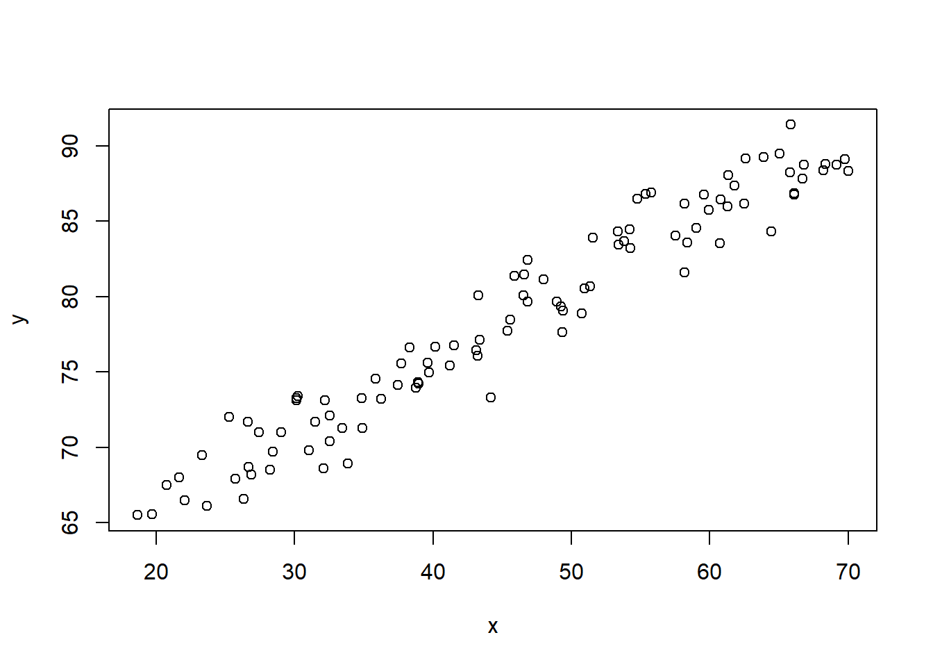
Suppose that we want to estimate the linear regression relationship between y and x at concurrent times.
Step 1: Estimate the usual regression model.
Results from R are:
Coefficients: Estimate Std. Error t value Pr(>|t|)
(Intercept) 57.76368214 3.84725610 15.0142545 4.816492e-27
trend 0.03449701 0.09415713 0.3663771 7.148816e-01
x 0.41798042 0.18859164 2.2163253 2.900638e-02Signif. codes: 0 '***' 0.001 '**' 0.01 '*' 0.05 '.' 0.1 ' ' 1Residual standard error: 1.774368 on 97 degrees of freedomMultiple R-squared: 0.9416116Adjusted R-squared: 0.9404078F-statistic: 782.1452 on 2 and 97 DF, p-value: NA Trend is not significant, however, we notice that x is increasing over time as well and is strongly correlated with time, r = .998. To reduce the multicollinearity between x and t, we can detrend x and examine the regression for y on the de-trended x, dtx, and time, t. The regression results are now:
Coefficients: Estimate Std. Error t value Pr(>|t|)
(Intercept) 66.2535494 0.357551977 185.297674 1.673616e-125
trend 0.2427347 0.006146899 39.488963 1.410780e-61
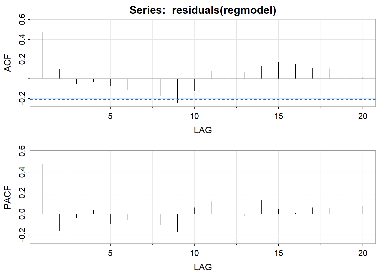
dtx 0.4179804 0.188591638 2.216325 2.900638e-02Signif. codes: 0 '***' 0.001 '**' 0.01 '*' 0.05 '.' 0.1 ' ' 1Residual standard error: 1.774368 on 97 degrees of freedomMultiple R-squared: 0.9416116Adjusted R-squared: 0.9404078 F-statistic: 782.1452 on 2 and 97 DF, p-value: NA Step 2: Examine the ARIMA structure of the residuals.
Following are the ACF and PACF of the residuals. Because both the ACF and PACF spike and then cut off, we should compare AR(1), MA(1), and ARIMA(1,0,1). We will continue with the MA(1) model in the notes.
Step 3: Estimate the adjusted model with a MA(1) structure for the residuals (and make sure that the MA model actually fits the residuals)
For this example, the R estimate of the model is
<><><><><><><><><><><><><><>

Coefficients:
          Estimate     SE  t.value p.value
ma1         0.4551 0.0753   6.0475  0.0000
intercept  66.2633 0.4489 147.6059  0.0000
trend       0.2423 0.0077  31.4466  0.0000
dtx         0.4364 0.1421   3.0711  0.0028

sigma^2 estimated as 2.380735 on 96 degrees of freedom

AIC = 3.807608  AICc = 3.811818  BIC = 3.937866
Step 4: Model diagnostics, (not shown here), suggested that the model fit well.
Thus our estimated relationship between \(y_t\) and \(x_t\) is
\[y_t = 66.26 + 0.24t + 0.44dtx_t + e_t\]
The errors have the estimated relationship \(e_t = w_t + 0.46w_{t−1}\) , where \(w_t\sim\text{iid}\; N(0,\sigma^2).\)
The R Program
Download the data used in the following code: (l8.1.x.dat), (l8.1.y.dat)
library(astsa)
x=ts(scan("l8.1.x.dat"))
y=ts(scan("l8.1.y.dat"))
plot(x,y, pch=20,main = "X versus Y")

trend = time(y)
regmodel=lm(y~trend+x) # first ordinary regression.
dtx = residuals(lm (x~time(x)))
regmodel= lm(y~trend+dtx) # first ordinary regression with detrended x, dtx.
summary(regmodel) # This gives us the regression results
acf2(resid(regmodel)) # ACF and PACF of the residuals

adjreg = sarima (y, 0,0,1, xreg=cbind(trend, dtx)) # This is the adjustment regression with MA(1) residuals
adjreg # Results of adjustment regression. White noise should be suggested.
acf2(resid(adjreg$fit))

library(nlme)
summary(gls(y ~ dtx+trend, correlation = corARMA(form = ~ 1,p=0,q=1))) #For comparison
Example 8.3 (Glacial Varve) Note that in this example it might work better to use an ARIMA model as we have a univariate time series, but we’ll use the approach of these notes for illustrative purposes. We analyze the glacial varve data described in Example 2.5 of the text. The response is a measure of the thickness of deposits of sand and silt (varve) left by spring melting of glaciers about 11,800 years ago. The data are annual estimates of varve thickness at a location in Massachusetts for 455 years beginning 11,834 years ago. There are nonconstant variance and outlier problems in the data, so we might try a log transformation with hopes of stabilizing the variance and diminishing the effects of outliers. Here’s a time series plot of the log10 series.
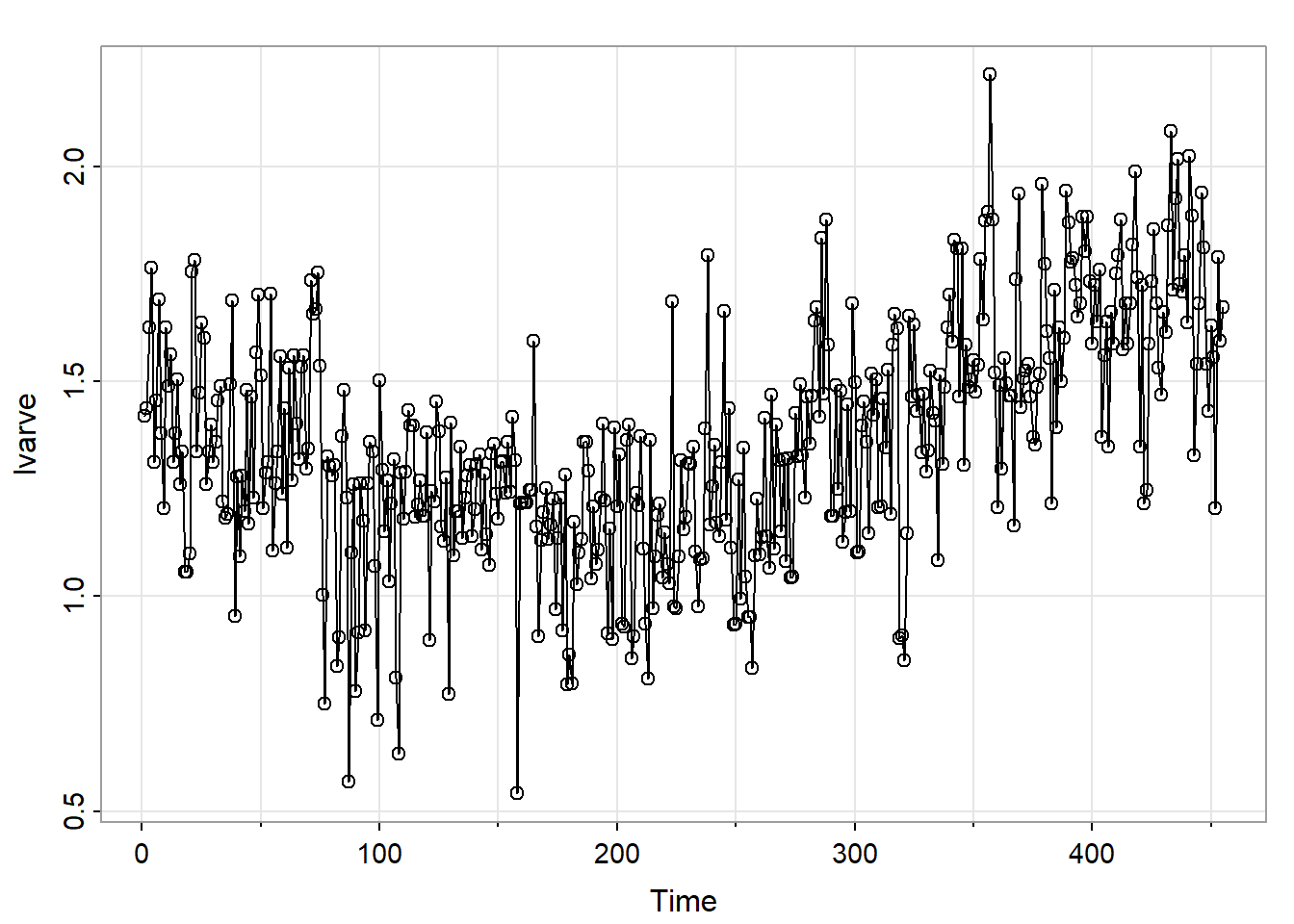
There’s a curvilinear pattern, so we’ll try the ordinary regression model
\[\text{log}_{10} y = \beta_0 + \beta_1 (t-\bar{t}) + \beta_2(t-\bar{t})^2 + \epsilon,\]
where \(t\) = year numbered 1, 2, …455.
Centering the time variable creates uncorrelated estimates of the linear and quadratic terms in the model. Regression results found using R are:
Call:
lm(formula = lvarve ~ trend + trend2)

Residuals:
     Min       1Q   Median       3Q      Max
-0.68884 -0.12418  0.01212  0.13195  0.74037

Coefficients:
             Estimate Std. Error t value Pr(>|t|)
(Intercept) 1.220e+00  1.502e-02   81.19   <2e-16 ***
trend       9.047e-04  7.626e-05   11.86   <2e-16 ***
trend2      8.283e-06  6.491e-07   12.76   <2e-16 ***
---
Signif. codes:  0 '***' 0.001 '**' 0.01 '*' 0.05 '.' 0.1 ' ' 1

Residual standard error: 0.2137 on 452 degrees of freedom
Multiple R-squared:  0.4018,    Adjusted R-squared:  0.3991
F-statistic: 151.8 on 2 and 452 DF,  p-value: < 2.2e-16
The autocorrelation and partial autocorrelation functions of the residuals from this model follow.
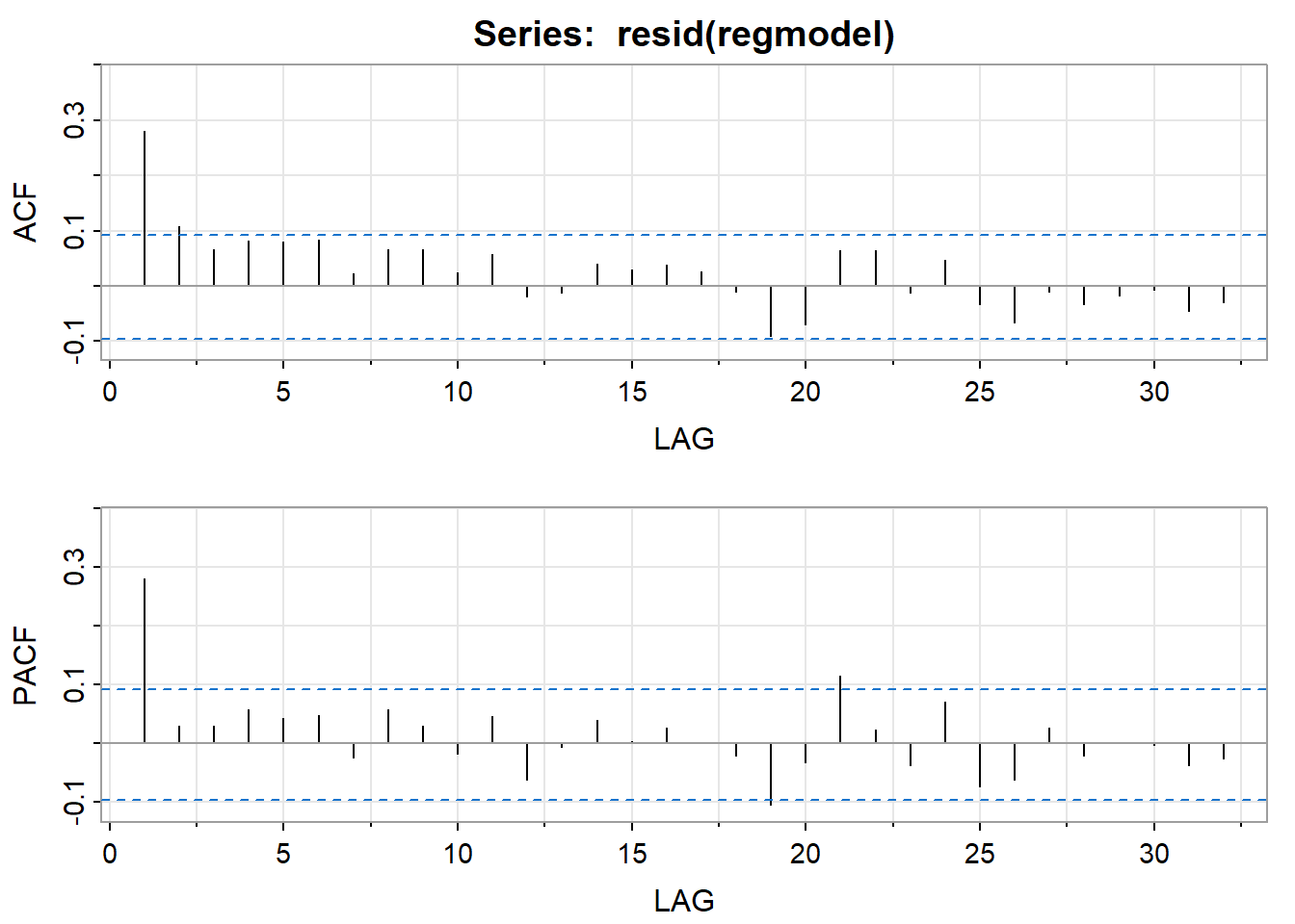
Similar to example 1, we might interpret the patterns either as an ARIMA(1,0,1), an AR(1), or a MA(1). We’ll pick the AR(1) – in large part to show an alternative to the MA(1) in Example 2.
The ARIMA results for a AR(1):
<><><><><><><><><><><><><><>

Coefficients:
          Estimate     SE t.value p.value
ar1         0.2810 0.0466  6.0290  0.0000
intercept   1.2202 0.0202 60.2954  0.0000
trend       0.0009 0.0001  8.0967  0.0000
trend2      0.0000 0.0000  0.1681  0.8666

sigma^2 estimated as 0.04175655 on 451 degrees of freedom

AIC = -0.315863  AICc = -0.3156676  BIC = -0.270585
NULLCheck diagnostics:
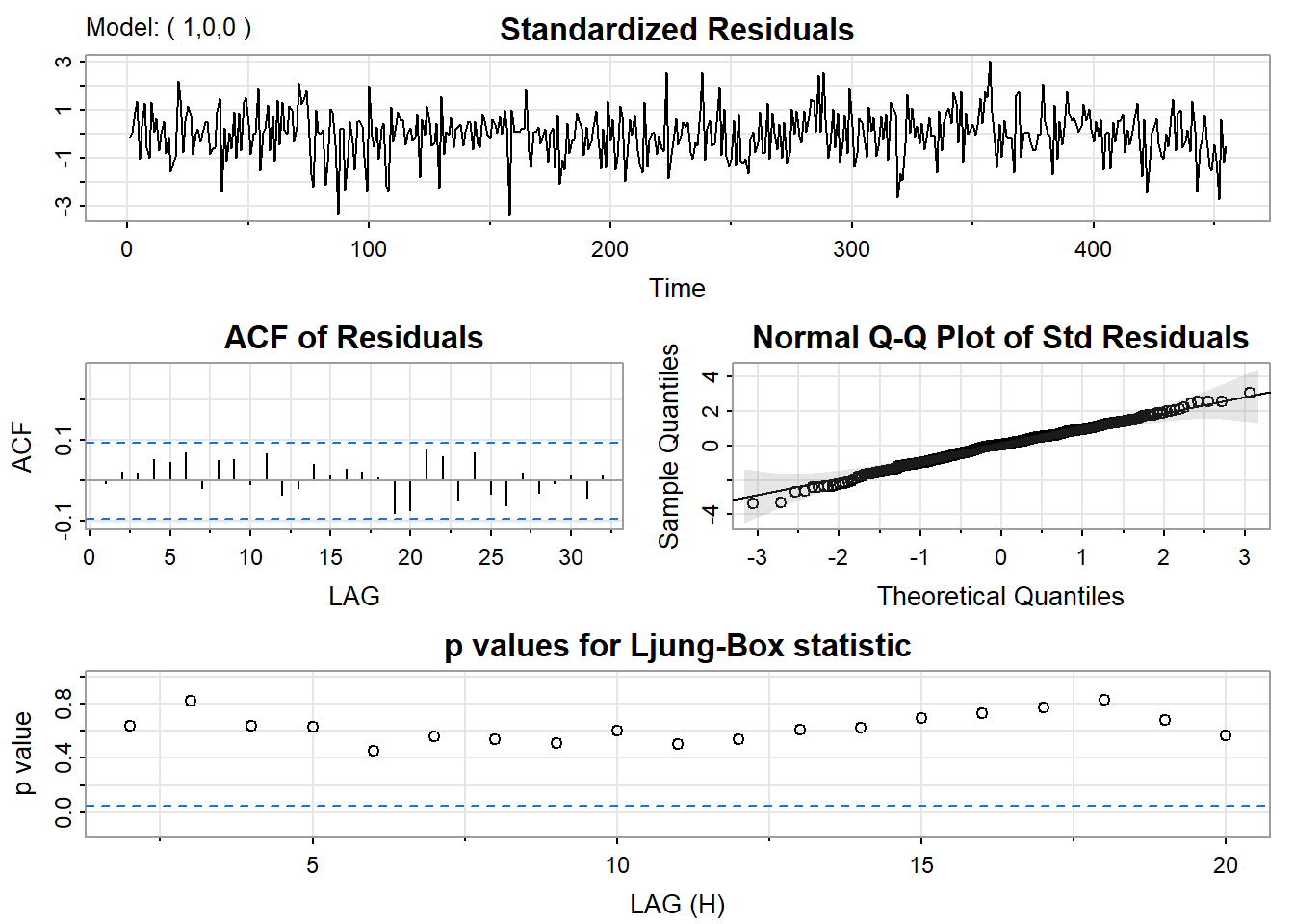
The autocorrelation and partial autocorrelation functions of the residuals from this estimated model include no significant values. The fit seems satisfactory, so we’ll use these results as our final model. The estimated model is
\[\text{log}_{10}y =1.22018 + 0.0009029(t − \bar{t}) + 0.00000826(t − \bar{t})^2,\]
with errors \(e_t = 0.2810 e_{t-1} +w_t\) and \(w_t \sim \text{iid} \; N(0,\sigma^2).\)
The R Program
The data are in varve.dat in the Week 8 folder, so you can reproduce this analysis or compare to a MA(1) for the residuals.
library(astsa)
varve=scan("varve.dat")
varve=ts(varve[1:455])
lvarve=log(varve,10)
trend = time(lvarve)-mean(time(lvarve))
trend2=trend^2
regmodel=lm(lvarve~trend+trend2) # first ordinary regression.
summary(regmodel)
acf2(resid(regmodel))
adjreg = sarima (lvarve, 1,0,0, xreg=cbind(trend,trend2)) #AR(1) for residuals
adjreg #Note that the squared trend is not significant, but should be kept for diagnostic purposes.
adjreg$fit$coef #Note that R actually prints 0’s for trend2 because the estimates are so small. This command prints the actual values.
8.2 Cross Correlation Functions and Lagged Regressions
The basic problem we’re considering is the description and modeling of the relationship between two time series.
In the relationship between two time series (\(y_{t}\) and \(x_{t}\)), the series \(y_{t}\) may be related to past lags of the x-series. The sample cross correlation function (CCF) is helpful for identifying lags of the x-variable that might be useful predictors of \(y_{t}.\)
In R, the sample CCF is defined as the set of sample correlations between \(x_{t+h}\) and \(y_{t}\) for h = 0, ±1, ±2, ±3, and so on. A negative value for \(h\) is a correlation between the x-variable at a time before \(t\) and the y-variable at time \(t.\) For instance, consider \(h\) = −2. The CCF value would give the correlation between \(x_{t-2}\) and \(y_{t}.\)
- When one or more \(x_{t+h}\) , with \(h\) negative, are predictors of \(y_{t},\) it is sometimes said that x leads y.
- When one or more \(x_{t+h},\) with \(h\) positive, are predictors of \(y_{t},\) it is sometimes said that x lags y.
In some problems, the goal may be to identify which variable is leading and which is lagging. In many problems we consider, though, we’ll examine the x-variable(s) to be a leading variable of the y-variable because we will want to use values of the x-variable to predict future values of y.
Thus, we’ll usually be looking at what’s happening at the negative values of \(h\) on the CCF plot.
Transfer Function Models
In a full transfer function model, we model \(y_{t}\) as potentially a function of past lags of \(y_{t}\) and current and past lags of the x-variables. We also usually model the time series structure of the x-variables as well. We’ll take all of that on next week. This week we’ll just look at the use of the CCF to identify some relatively simple regression structures for modeling \(y_{t}.\)
Sample CCF in R
The CCF command is
ccf(x-variable name, y-variable name)If you wish to specify how many lags to show, add that number as an argument of the command. For instance, ccf(x,y, 50) will give the CCF for values of \(h\) = 0, ±1, …, ±50.
Example 8.4 (Southern Oscillation Index and Fish Populations in the southern hemisphere.) The text describes the relationship between a measure of weather called the Southern Oscillation Index (SOI) and “recruitment,” a measure of the fish population in the southern hemisphere. The data are monthly estimates for n = 453 months. We see SOI as a potential predictor of recruit.
The data are in two different files. The CCF below was created with these commands:
soi= scan("soi.dat")
rec = scan("recruit.dat")
soi=ts (soi)
rec = ts(rec)
ccf (soi, rec) 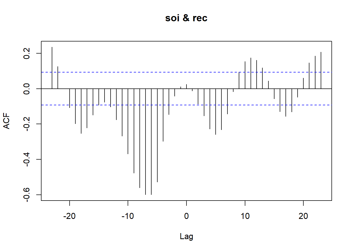
The most dominant cross correlations occur somewhere between \(h =−10\) and about \(h = −4.\) It’s difficult to read the lags exactly from the plot, so we might want to give an object name to the ccf and then list the object contents. The following two commands will do that for our example.
ccfvalues = ccf(soi,rec)
ccfvalues
The output shows the correlation with \((y_t)\) for each lag, that is the \((h)\) in \((x_{t+h})\):
Autocorrelations of series 'X', by lag
-23 -22 -21 -20 -19 -18 -17 -16 -15 -14 -13
0.235 0.125 0.000 -0.108 -0.198 -0.253 -0.222 -0.149 -0.092 -0.076 -0.103
-12 -11 -10 -9 -8 -7 -6 -5 -4 -3 -2
-0.175 -0.267 -0.369 -0.476 -0.560 -0.598 -0.599 -0.527 -0.297 -0.146 -0.042
-1 0 1 2 3 4 5 6 7 8 9
0.011 0.025 -0.013 -0.086 -0.154 -0.228 -0.259 -0.232 -0.144 -0.017 0.094
10 11 12 13 14 15 16 17 18 19 20
0.154 0.174 0.162 0.118 0.043 -0.057 -0.129 -0.156 -0.131 -0.049 0.060
21 22 23
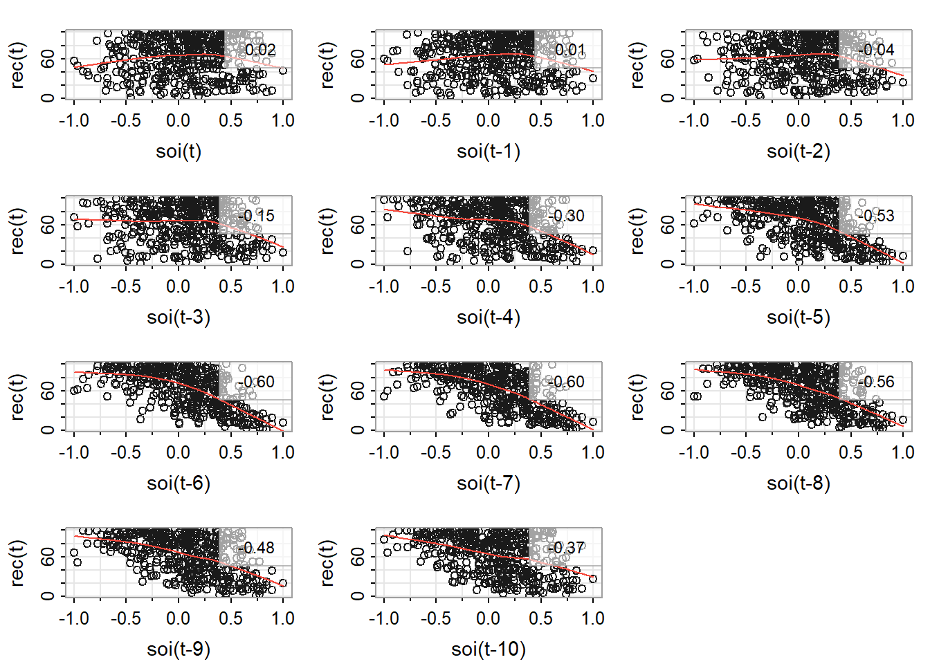
0.147 0.184 0.206 There are nearly equal maximum values at \(h\) = −5, −6, −7, and −8 with tapering occurring in both directions from that peak.
Scatterplots
In the astsa library that we’ve been using, Stoffer included a script that produces scatterplots of \(y_t\) versus \(x_{t+h}\) for negative \(h\) from 0 back to a lag that you specify. The command is lag2.plot.
The result of the command lag2.plot (soi, rec, 10) is shown below. In each plot, (recruit variable) is on the vertical and a past lag of SOI is on the horizontal. Correlation values are given on each plot.
Regression Models
There are a lot of models that we could try based on the CCF and lagged scatterplots for these data. For demonstration purposes, we’ll first try a multiple regression in which \(y_t,\) the recruit variable, is a linear function of (past) lags 5, 6, 7, 8, 9, and 10 of the SOI variable. That model works fairly well. Following is some R output. All coefficients are statistically significant and the R-squared is about 62%.
The residuals, however, have an AR(2) structure, as seen in the graph following the regression output. We might try the method described in Lesson 8.1 to adjust for that, but we’ll take a different approach that we’ll describe after the output display.
Call:
lm(formula = rec ~ soilag5 + soilag6 + soilag7 + soilag8 + soilag9 +
    soilag10, data = alldata)

Residuals:
    Min      1Q  Median      3Q     Max
-69.199 -11.593   1.143  12.946  34.494

Coefficients:
            Estimate Std. Error t value Pr(>|t|)
(Intercept)  69.2743     0.8703  79.601  < 2e-16 ***
soilag5     -23.8255     2.7657  -8.615  < 2e-16 ***
soilag6     -15.3775     3.1651  -4.858 1.65e-06 ***
soilag7     -11.7711     3.1665  -3.717 0.000228 ***
soilag8     -11.3008     3.1664  -3.569 0.000398 ***
soilag9      -9.1525     3.1651  -2.892 0.004024 **
soilag10    -16.7219     2.7693  -6.038 3.33e-09 ***
---
Signif. codes:  0 '***' 0.001 '**' 0.01 '*' 0.05 '.' 0.1 ' ' 1

Residual standard error: 17.42 on 436 degrees of freedom
Multiple R-squared:  0.6251,    Adjusted R-squared:   0.62
F-statistic: 121.2 on 6 and 436 DF,  p-value: < 2.2e-16
Next lesson we’ll discuss more about ways to interpret the CCF. One feature that will be described in more detail (with the “why”) is that a peak in a CCF followed by a tapering pattern is an indicator that lag 1 and possibly lag 2 values of the y-variable may be helpful predictors.
So, our try number 2 for a regression model will be to use lag 1 and lag 2 values of the y-variable as well as lags 5 through 10 of the x-variable as linear predictors. Here’s the outcome:
Call:
lm(formula = rec ~ reclag1 + reclag2 + soilag5 + soilag6 + soilag7 +
    soilag8 + soilag9 + soilag10, data = alldata)

Residuals:
    Min      1Q  Median      3Q     Max
-52.467  -2.855  -0.043   3.107  28.421

Coefficients:
             Estimate Std. Error t value Pr(>|t|)
(Intercept)  11.43047    1.33384   8.570  < 2e-16 ***
reclag1       1.25702    0.04316  29.128  < 2e-16 ***
reclag2      -0.41946    0.04120 -10.182  < 2e-16 ***
soilag5     -21.19210    1.11838 -18.949  < 2e-16 ***
soilag6       9.77648    1.56238   6.257  9.4e-10 ***
soilag7      -1.19189    1.32247  -0.901   0.3679
soilag8      -2.17345    1.30806  -1.662   0.0973 .
soilag9       0.56520    1.30035   0.435   0.6640
soilag10     -2.58630    1.19529  -2.164   0.0310 *
---
Signif. codes:  0 '***' 0.001 '**' 0.01 '*' 0.05 '.' 0.1 ' ' 1

Residual standard error: 7.034 on 434 degrees of freedom
Multiple R-squared:  0.9392,    Adjusted R-squared:  0.938
F-statistic: 837.5 on 8 and 434 DF,  p-value: < 2.2e-16
The R-squared value has gone to about 94%. Not all sample coefficients are statistically significant. Although it’s dangerous to drop too much from a model at once, we now see that lags 7 and above are not integral predictors in the presence of the other terms. Let’s drop lags 7, 8 , 9, and maybe 10 of SOI from the model. You might disagree with dropping lag 10 of SOI, but we’ll try it because it seems odd to have a “stray” term like that. .
So our third attempt is to predict \(y_t\) using lags 1 and 2 of itself and lags 5 and 6 of the x-variable (SOI). Here’s what happens:
Call:
lm(formula = rec ~ reclag1 + reclag2 + soilag5 + soilag6, data = alldata)
Residuals:
Min 1Q Median 3Q Max
-53.786 -2.999 -0.035 3.031 27.669
Coefficients:
Estimate Std. Error t value Pr(>|t|)
(Intercept) 8.78498 1.00171 8.770 < 2e-16 ***
reclag1 1.24575 0.04314 28.879 < 2e-16 ***
reclag2 -0.37193 0.03846 -9.670 < 2e-16 ***
soilag5 -20.83776 1.10208 -18.908 < 2e-16 ***
soilag6 8.55600 1.43146 5.977 4.68e-09 ***
---
Signif. codes: 0 '***' 0.001 '**' 0.01 '*' 0.05 '.' 0.1 ' ' 1
Residual standard error: 7.069 on 442 degrees of freedom
Multiple R-squared: 0.9375, Adjusted R-squared: 0.937
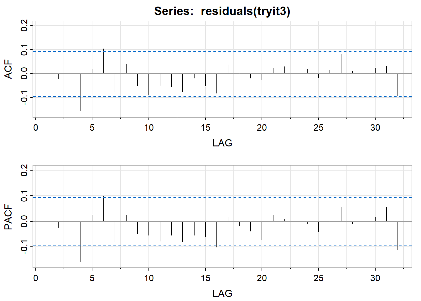
F-statistic: 1658 on 4 and 442 DF, p-value: < 2.2e-16All sample coefficients are significant and the R-squared is still about 94%. The ACF and PACF of the residuals look pretty good. There’s a barely significant residual autocorrelation at lag 4 which we may or may not want to worry about.
Complications
The CCF pattern is affected by the underlying time series structures of the two variables and the trend each series has. It often (perhaps most often) is helpful to de-trend and/or take into account the univariate ARIMA structure of the x-variable before graphing the CCF. We’ll play with this a bit in the homework this week and will take it on more fully next week.
R Code
Here’s the full R code for this handout. The alldata=ts.intersect() command preserves proper alignment between all of the lagged variables (and defines lagged variables). The tryit=lm() commands are specifying the various regression models and saving results as named objects.
Download the data used the following code: (soi.dat), (recruit.dat)
library(astsa)
soi= scan("soi.dat")
rec = scan("recruit.dat")
soi=ts (soi)
rec = ts(rec)
ccfvalues =ccf (soi, rec)
ccfvalues
lag2.plot (soi, rec, 10)
alldata=ts.intersect(rec,reclag1=lag(rec,-1), reclag2=lag(rec,-2), soilag5 = lag(soi,-5),
soilag6=lag(soi,-6), soilag7=lag(soi,-7), soilag8=lag(soi,-8), soilag9=lag(soi,-9),
soilag10=lag(soi,-10))
tryit = lm(rec~soilag5+soilag6+soilag7+soilag8+soilag9+soilag10, data = alldata)
summary (tryit)
acf2(residuals(tryit))
tryit2 = lm(rec~reclag1+reclag2+soilag5+soilag6+soilag7+soilag8+soilag9+soilag10,
data = alldata)
summary (tryit2)
acf2(residuals(tryit2))
tryit3 = lm(rec~reclag1+reclag2+ soilag5+soilag6, data = alldata)
summary (tryit3)
acf2(residuals(tryit3))