Printer-friendly version

• The linear regression model

\[ f(X)=\beta_{0} + \sum_{j=1}^{p}X_{j}\beta_{j}\]

This is just a linear combination of the measurements that are used to make predictions, plus a constant, (the intercept term). This is a simple approach. However, It might be the case that the regression function might be pretty close to a linear function, and hence the model is a good approximation.

What if the model is not true?

• It still might be a good approximation - the best we can do.
• Sometimes because of the lack of training data or smarter algorithms, this is the most we can estimate robustly from the data.

Comments on X_j :

• We assume that these are quantitative inputs [or dummy indicator variables representing levels of a qualitative input]
• We can also perform transformations of the quantitative inputs, e.g., log(•), √(•). In this case, this linear regression model is still a linear function in terms of the coefficients to be estimated. However, instead of using the original X_j, we have replaced them or augmented them with the transformed values. Regardless of the transformations performed on X_j, f(X) is still a linear function of the unknown parameters.
• Some basic expansions: X₂ = X₁² , X₃ = X₁³ , X₄ = X1 • X2.

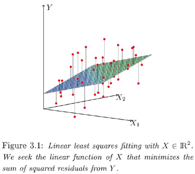
Below is a geometric interpretation of a linear regression.

For instance, if we have two variables, X₁ and X₂, and we predict Y by a linear combination of X₁ and X₂, the predictor function corresponds to a plane (hyperplane) in the three-dimensional space of X₁, X₂, Y. Given a pair of X₁ and X₂ we could find the corresponding point on the plane to decide Y by drawing a perpendicular line to the hyperplane, starting from the point in the plane spanned by the two predictor variables.

For accurate prediction, hopefully the data will lie close to this hyperplane, but they won't lie exactly in the hyperplane (unless perfect prediction is achieved). In the plot above, the red points are the actual data points. They do not lie on the plane but are close to it.

How should we choose this hyperplane?

We choose a plane such that the total squared distance from the red points (real data points) to the corresponding predicted points in the plane is minimized. Graphically, if we add up the squares of the lengths of the line segments drawn from the red points to the hyperplane, the optimal hyperplane should yield the minimum sum of squared lengths.

Estimation

The issue of finding the regression function E(Y | X) is converted to estimating β_j , j = 0, 1, ..., p.

Remember in earlier discussions we talked about the trade-off between model complexity and accurate prediction on training data. In this case, we start with a linear model, which is relatively simple. The model complexity issue is taken care of by using a simple linear function. In basic linear regression, there is no explicit action taken to restrict model complexity. [Although variable selection, which we cover in Lesson 4, can be considered a way to control model complexity.]

With the model complexity under check, the next thing we want to do is to have a predictor that fits the training data well.

Let the training data be:

{(x₁, y₁), (x₂, y₂), ..., (x_N, y_N )}, where x_i = (x_i1, x_i2, ..., x_ip).

Denote β = (β₀, β₁, ..., β_p)^T .

Without knowing the true distribution for X and Y, we cannot directly minimize the expected loss.

Instead, the expected loss E(Y − f(X))² is approximated by the empirical loss RSS(β)/N :

\( \begin {align}RSS(\beta)&=\sum_{i=1}^{N}\left(y_i - f(x_i)\right)^2 \\  &=\sum_{i=1}^{N}\left(y_i - \beta_0 -\sum_{j=1}^{p}x_{ij}\beta_{j}\right)^2  \\ \end {align}  \)

This empirical loss is basically the accuracy you computed based on the training data. This is called the residual sum of squares, RSS.

The x's are known numbers from the training data.

Notation

Here is the input matrix X of dimension N × (p +1):

\begin{pmatrix}
1 & x_{1,1}  &x_{1,2}  & ... &x_{1,p} \\
1 & x_{2,1} & x_{2,2} & ... &x_{2,p} \\
... & ... & ... & ...  & ... \\
1 & x_{N,1} &x_{N,2} &...  & x_{N,p}
\end{pmatrix}

Earlier we mentioned that our training data had N number of points. So, in the example where we were predicting the number of doctors, there were 101 metropolitan areas that were investigated. Therefore, N =101. Dimension p = 3 in this example. The input matrix is augmented with a column of 1's (for the intercept term). So, above you see the first column contains all 1's. Then if you look at every row, every row corresponds to one sample point and the dimensions go from one to p. Hence, the input matrix X is of dimension N × (p +1).

Output vector y:

\[ y= \begin{pmatrix}
y_{1}\\
y_{2}\\
...\\
y_{N}
\end{pmatrix} \]

Again, this is taken from the training data set.

The estimated β is \(\hat{\beta}\) and this is also put in a column vector, (β₀, β₁, ..., β_p).

The fitted values (not the same as the true values) at the training inputs are

\[\hat{y}_{i}=\hat{\beta}_{0}+\sum_{j=1}^{p}x_{ij}\hat{\beta}_{j}\]

and

\[ \hat{y}= \begin{pmatrix}
\hat{y}_{1}\\
\hat{y}_{2}\\
...\\
\hat{y}_{N}
\end{pmatrix} \].

For instance, if you are talking about sample i, the fitted value for sample i would be to take all the values of the x's for sample i, (denoted by x_ij) and do a linear summation for all of these x_ij's with weights \(\hat{\beta}_{j}\) and the intercept term \(\hat{\beta}_{0}\).